1. Basic Renderer
A renderer is a collection of algorithms that take a Scene data
structure as its input and produces a FrameBuffer data structure
as its output.
                           Renderer
                       +--------------+
       Scene           |              |         FrameBuffer
       data     ====>  |  Rendering   |  ====>     data
     structure         |  algorithms  |          structure
                       |              |
                       +--------------+
A Scene data structure contains information that describes a "virtual
scene" that we want to take a "picture" of. The renderer is kind of like
a digital camera and the FrameBuffer is the camera's film. The renderer
takes (calculates) a picture of the Scene and stores the picture in the
FrameBuffer. The FrameBuffer holds the pixel information that describes
the picture of the virtual scene.
The rendering algorithms can be implemented in hardware (a graphics card or a GPU) or in software. In this class we will write a software renderer using the Java programming language.
Our software renderer is made up of four "packages" of Java classes. Each package is contained in its own directory. The name of the directory is the name of the package.
The first package is the collection of input data structures. This is called
the scene package. The data structure files in the scene package are:
- Scene.java
- Camera.java
- Position.java
- Vector.java
- Model.java
- Primitive.java
- LineSegment.java
- Point.java
- Vertex.java
The Primitive, LineSegment, and Point classes are in a sub-package
called primitives.
The second package is the output data structure. It is called the
framebuffer package and contains the file
- FrameBuffer.java.
The third package is a collection of algorithms that manipulate the
data structures from the other two packages. This package is called
the pipeline package. The algorithm files are:
- Pipeline.java
- Model2Camera.java
- Projection.java
- Viewport.java
- Rasterize.java
- Rasterize_Clip_AntiAlias_Line.java
- Rasterize_Clip_Point.java
The fourth package is a library of geometric models. This package is
called the models_L package. It contains a number of files for geometric
shapes such as sphere, cylinder, cube, cone, pyramid, tetrahedron,
dodecahedron, and mathematical curves and surfaces.
There is also a fifth package, a collection of client programs that use
the renderer. These files are in a folder called clients_r1.
Here is a brief description of the data structures from the scene and
framebuffer packages.
-
A
FrameBufferobject represents a two-dimensional array of pixel data. Pixel data represents the red, green, and blue colors of each pixel in the image that the renderer produces. TheFrameBufferalso defines a two-dimensional sub-array of pixel data called aViewport. -
A
Sceneobject has aCameraobject and aListofPositionobjects. -
A
Cameraobject has a boolean which determines if the camera is a perspective camera or an orthographic camera. -
A
Positionobject has aVectorobject and aModelobject. -
A
Vectorobject has three doubles, the x, y, z coordinates of a vector in 3-dimensional space. AVectorrepresents a location in 3-dimensional space, the location of theModelthat is in aPositionwith theVector. -
A
Modelobject has aListofVertexobjects, aLIstofColorobjects, and aListofPrimitiveobjects. -
A
Vertexobject has three doubles, the x, y, z coordinates of a point in 3-dimensional space. -
A
Colorobject represents the red, green, can blue components of a color. We will use Java's built inColorclass. -
A
Primitiveobject is either aLineSegmentobject or aPointobject. -
A
LineSegmentobject has two lists of two integers each. The two integers in the firstListare indices into theModel'sListof vertices. This lets aLineSegmentobject represent the two endpoints of a line segment in 3-dimensional space. The two integers in the secondListare indices into theModel'sListof colors, one color for each endpoint of the line segment. -
A
Pointobject has three integer values. The first integer is an index into theModel'sListof vertices. This lets aPointobject represent a single point in 3-dimensional space. The second integer is an index into theModel'sListof colors. The third integer is the "diameter" of the point, which lets thePointbe visually represented by a block of pixels.
1.1 Scene tree data structure
When we put all of the above information together, we see that
a Scene object is the root of a tree data structure.
            Scene
           /     \
          /       \
    Camera        List<Position>
                   /     |      \
                  /      |       \
          Position    Position    Position
           /    \     /       \    /    \
                     /         \
                    /           \
              Vector             Model
              / | \             /  |  \
             x  y  z       /---/   |   \---\
                          /        |        \
                         /         |         \
              List<Vertex>    List<Color>     List<Primitive>
                /   |   \      /   |   \          /   |   \
                    |              |                  |
                 Vertex          Color             LineSegment
                  / | \          / | \            /           \
                 x  y  z        r  g  b          /             \
                                          List<Integer>     List<Integer>
                                            (vertices)        (colors)
                                             /     \           /    \
                                            /       \         /      \
                                        Integer  Integer   Integer  Integer
In the renderer.scene.util package there is a file called DrawSceneGraph.java
that can create image files containing pictures of a scene's tree data
structure. The pictures of the tree data structures are actually created
by a program called GraphViz. If you want the renderer to be able to draw
these pictures, then you need to install GraphViz on your computer.
https://en.wikipedia.org/wiki/Scene_graph
1.2 Renderer source code
The Java source code to this renderer is publicly available as a zip file.
Here is a link to the renderer's source code.
http://cs.pnw.edu/~rlkraft/cs45500/for-class/renderer_1.zip
Download and unzip the source code to any convenient location in your computer's file system. The renderer does not have any dependencies other than the Java 11 (or later) JDK (Java Development Kit). So once you have downloaded and unzipped the distribution, you are ready to compile the renderer and run the renderer's example programs.
The following sections of this document describe the organization of the renderer packages and provide instructions for building the renderer and its client programs.
https://openjdk.org/projects/jdk/11/
2. Packages, imports, classpath
Before we go into the details of each renderer package, let us review some of the details of how the Java programming language uses packages.
But first, let us review some of the details of how Java classes are defined and how the Java compiler compiles them.
A Java class is defined in a text file with the same name as the class and with the filename extension ".java". When the compiler compiles the class definition, it produces a binary (machine readable) version of the class and puts the binary code in a file with the same name as the class but with the file name extension ".class".
Every Java class will make references to other Java classes. For example,
here is a simple Java class called SimpleClass that should be stored in
a text file called SimpleClass.java.
import java.util.Scanner;

public class SimpleClass {
   public static void main(String[] args) {
      final Scanner in = new Scanner(System.in);
      final int n = in.nextInt();
      System.out.println(n);
   }
}
This class refers to the Scanner class, the String class, the System
class, the InputStream class (why?), the PrintStream class (why?), and, in
fact, many other classes. When you compile the source file SimpleClass.java,
the compiler produces the binary file SimpleClass.class. As the compiler
compiles SimpleClass.java, the compiler checks for the existence of all
the classes referred to by SimpleClass.java. For example, while compiling
SimpleClass.java the compiler looks for the file Scanner.class. If it
finds it, the compiler continues with compiling SimpleClass.java (after
the compiler makes sure that your use of Scanner is consistent with the
definition of the Scanner class). But if Scanner.class is not found, then
the compiler looks for the text file Scanner.java. If the compiler finds
Scanner.java, the compiler compiles it to produce Scanner.class, and then
continues with compiling SimpleClass.java. If the compiler cannot find
Scanner.java, then you get a compiler error from compiling SimpleClass.java.
The same goes for all the other classes referred to by SimpleClass.java.
Here is an important question. When the compiler sees, in the compiling of
SimpleClass.java, a reference to the Scanner class, how does the compiler
know where it should look for the files Scanner.class or Scanner.java?
These files could be anywhere in your computer's file system. Should the
compiler search your computer's entire storage drive for the Scanner
class? The answer is no, for two reasons (one kind of obvious and one kind
of subtle). The obvious reason is that the computer's storage drive is very
large and searching it is time consuming. If the compiler has to search your
entire drive for every class reference, it will take way too long to compile
a Java program. The subtle reason is that it is common for computer systems
to have multiple versions of Java stored in the file system. If the compiler
searched the whole storage drive for classes, it might find classes from
different versions of Java and then try to use them together, which does
not work. All the class files must come from the same version of Java.
The compiler needs help in finding Java classes so that it only looks in certain controlled places in the computer's file system and so that it does not choose classes from different versions of Java.
The import statements at the beginning of a Java source file are part of the solution to helping the compiler find class definitions.
An import statement tells the Java compiler how to find a class
definition. In SimpleClass.java, the import statement
import java.util.Scanner;
tells the compiler to find a folder named java and then within that folder
find a folder named util and then within that folder find a class file
named Scanner.class (or a source file named Scanner.java).
The folders in an import statement are called packages. In Java, a package is a folder in your computer's file system that contains a collection of Java class files or Java source files. The purpose of a package is to organize Java classes. In a large software project there will always be many classes. Having all the classes from a project (maybe thousands of them) in one folder would make understanding the project's structure and organization difficult. Combining related classes into a folder helps make the project's structure clearer.
The import statement
import java.util.Scanner;
tells us (and the compiler) that Java has a package named java and a
sub-package named java.util. The Scanner class is in the package
java.util (notice that the package name is java.util, not util).
Look at the Javadoc for the Scanner class.
https://docs.oracle.com/en/java/javase/21/docs/api/java.base/java/util/Scanner.html
The very beginning of the documentation page tells us the package that this class is in.
What about the class String? Where does the compiler look for the String
class? Notice that there is no import statement for the String class. Look
at the Javadoc for the String class.
https://docs.oracle.com/en/java/javase/21/docs/api/java.base/java/lang/String.html
The String class is in a package named java.lang. The java.lang package
is automatically imported for us by the Java compiler. This package contains
classes that are so basic to the Java language the all Java programs will
need them, so these classes are all placed in one package and that package
gets automatically imported by the Java compiler.
We still haven't fully explained how the Java compiler finds the Scanner
class. The import statement
import java.util.Scanner;
tells the compiler to find a folder called java and the Scanner class
will be somewhere inside that folder. But where does the compiler find
the java folder? Should it search your computer's entire file system
for a folder called java? Obviously not, but we seem to be right back
to the problem that we started with. Where does the compiler look in your
computer's file system? The answer is another piece of the Java system,
something called the "classpath".
The classpath is a list of folder names that the compiler starts its search from when it searches for a package. A classpath is written as a string of folder names separated by semicolons (or colons on a Linux computer). A Windows classpath might look like this.
C:\myProject;C:\yourLibrary\utils;D:\important\classes
This classpath has three folder names in its list. A Linux classpath might look like this.
/myProject:/yourLibrary/utils:/important/classes
When you compile a Java source file, you can specify a classpath on the compiler command-line.
> javac -cp C:\myProject;C:\yourLibrary\utils;D:\important\classes MyProgram.java
The Java compiler will only look for packages that are subfolders of the folders listed in the classpath.
The Java compiler has some default folders that it always uses as part of
the classpath, even if you do not specify a value for the classpath. The
JDK that you install on your computer is always part of the compiler's
classpath. So Java packages like java.lang and java.util (and many
other packages), which are part of the JDK, are always in the compiler's
classpath.
If you do not specify a classpath, then the compiler's default classpath will include the directory containing the file being compiled (the current directory). However, if you DO specify a classpath, then the compiler will NOT automatically look in the current directory. Usually, when someone gives the compiler a classpath, they explicitly include the "current directory" in the classpath list. In a classpath, the name you use for the "current directory" is a single period, ".". So a classpath that explicitly includes the current directory might look like this.
> javac -cp .;C:\myProject;C:\yourLibrary\utils;D:\important\classes MyProgram.java
You can put the . anywhere in the classpath, but most people put it at the
beginning of the classpath to make it easier to read. A common mistake is to
specify a classpath but forget to include the current directory in it.
Here is an example of an import statement from our renderer.
import renderer.scene.util.DrawSceneGraph;
This import statement says that there is a folder named renderer with
a subfolder named scene with a subfolder named util that contains a
file named DrawSceneGraph.java (or DrawSceneGraph.class). The file
DrawSceneGraph.java begins with a line of code called a package
statement.
package renderer.scene.util;
A package statement must come before any import statements.
A class file contains a "package statement" declaring where that class file should be located. Any Java program that wants to use that class (a "client" of that class) should include an "import statement" that matches the "package statement" from the class. When the client is compiled, we need to give the compiler a "classpath" that tells the compiler where to find the folders named in the import statements.
A Java class is not required to have a package statement. A class without a package statement becomes part of a special package called the unnamed package. The unnamed package is always automatically imported by the compiler. The unnamed package is used mostly for simple test programs or simple programs demonstrating an idea, or examples programs in introductory programming courses. The unnamed package is never used for library classes or classes that need to be shared as part of a large project.
A Java class file is not required to have any import statements. You can
use any class you want without having to import it. But if you use a class
without importing it, then you must always use the full package name
for the class. Here is an example. If we import the Scanner class,
import java.util.Scanner;
The we can use the Scanner class like this.
final Scanner in = new Scanner(System.in);
But if we do not import the Scanner class, then we can still use it,
but we must always refer to it by its full package name, like this.
final java.util.Scanner in = new java.util.Scanner(System.in);
If you are using a class in many places in your code, then you should import it. But if you are referring to a class in just a single place in your code, then you might choose to not import it and instead use the full package name for the class.
We can import Java classes using the wildcard notation. The following
import statement imports all the classes in the java.util package,
including the Scanner class.
import java.util.*;
There are advantages and disadvantages to using wildcard imports. One
advantage is brevity. If you are using four classes from the java.util
package, then you need only one wildcard import instead of four fully
qualified imports.
One disadvantage is that wildcard imports can lead to name conflicts.
The following program will not compile because both the java.util and
the java.awt packages contain a class called List. And both the
java.util and the java.sql packages contain a class called Date.
import java.util.*; // This package contains a List and a Date class.
import java.awt.*;  // This package contains a List class.
import java.sql.*;  // This package contains a Date class.

public class Problem {
   public static void main(String[] args) {
      List list = null;  // Which List class?
      Date date = null;  // Which Date class?
   }
}
We can solve this problem by combining a wildcard import with a qualified import.
import java.util.*; // This package contains a List and a Data class.
import java.awt.*;  // This package contains a List class.
import java.sql.*;  // This package contains a Date class.
import java.awt.List;
import java.sql.Date;

public class ProblemSolved {
   public static void main(String[] args) {
      List list = null;  // From java.awt package.
      Date date = null;  // From java.sql package.
   }
}
You can try compiling these last two examples with the Java Visualizer.
https://cscircles.cemc.uwaterloo.ca/java_visualize/
If you want to see more examples of using packages and classpaths, look at the code in the follow zip file.
http://cs.pnw.edu/~rlkraft/cs45500/for-class/package-examples.zip
There is more to learn about how the Java compiler finds and compiles Java classes. For example, we have not yet said anything about jar files. Later we will see how, and why, we use jar files.
https://dev.java/learn/packages/
https://docs.oracle.com/javase/tutorial/java/package/index.html https://docs.oracle.com/javase/tutorial/java/package/QandE/packages-questions.html https://docs.oracle.com/javase/tutorial/deployment/jar/basicsindex.html
https://en.wikipedia.org/wiki/Classpath
https://docs.oracle.com/javase/specs/jls/se17/html/jls-7.html#jls-7.4.2 https://docs.oracle.com/javase/8/docs/technotes/tools/findingclasses.html
https://en.wikipedia.org/wiki/JAR_(file_format) https://dev.java/learn/jvm/tools/core/jar/
3. Build System
Any project as large as this renderer will need some kind of "build system".
https://en.wikipedia.org/wiki/Build_system_(software_development)
The renderer has over 100 Java source files. To "build" the renderer we need to produce a number of different "artifacts" such as class files, HTML Javadoc files, jar files. We do not want to open every one of the 100 or so Java source code files and compile each one. We need a system that can automatically go through all the sub folders of the renderer and compile every Java source file to a class file, produce the Javadoc HTML files, and then bundle the results into jar files.
Most Java projects use a build system like Maven, Gradle, Ant, or Make.
In this course we will use a much simpler build system consisting of
command-line script files (cmd files on Windows and bash files on
Linux). We will take basic Java command-lines and place them in the
script files. Then by running just a couple of script files, we can
build all the artifacts we need.
We will write script files for compiling all the Java source files (using
the javac command), creating all the Javadoc HTML files (using the javadoc
command), running individual client programs (using the java command), and
bundling the renderer library into jar files (using the jar command). We
will also write script files to automatically "clean up" the renderer folders
by deleting all the artifacts that the build scripts generate.
Here are help pages for the command-line tools that we will use.
- https://dev.java/learn/jvm/tools/core/
- https://dev.java/learn/jvm/tools/core/javac/
- https://dev.java/learn/jvm/tools/core/java/
- https://dev.java/learn/jvm/tools/core/javadoc/
- https://dev.java/learn/jvm/tools/core/jar/
Be sure to look at the contents of all the script files. Most are fairly simple. Understanding them will help you understand the more general build systems used in industry.
There are two main advantages of using such a simple build system.
- No need to install any new software (we use Java's built-in tools).
- It exposes all of its inner workings (nothing is hidden or obscured).
Here are the well known build systems used for large projects.
- https://maven.apache.org/
- https://gradle.org/
- https://ant.apache.org/
- https://www.gnu.org/software/make/
Here is some documentation on the Windows cmd command-line language
and the Linux bash command-line language.
- https://linuxcommand.org/lc3_learning_the_shell.php
- https://learn.microsoft.com/en-us/windows-server/administration/windows-commands/windows-commands
- https://ss64.com/nt/syntax.html
3.1 Building class files
Here is the command line that compiles all the Java files in the scene
package.
> javac -g -Xlint -Xdiags:verbose renderer/scene/*.java
This command-line uses the Java compiler command, javac. The javac
command, like almost all command-line programs, takes command-line arguments
(think of "command-line programs" as functions and "command-line arguments"
as the function's parameters). The -g is the command-line argument that
tells the compiler to produce debugging information so that we can debug
the renderer's code with a visual debugger. The -Xlint is the command-line
argument that tells the compiler to produce all possible warning messages
(not just error messages). The -Xdiags:verbose command-line argument tells
the compiler to put as much information as it can into each error or warning
message. The final command-line argument is the source file to compile. In
this command-line we use file name globbing to compile all the .java
files in the scene folder.
There are a large number of command-line arguments that we can use with the
javac command. All the command-line arguments are documented in the help
page for the javac command.
https://docs.oracle.com/en/java/javase/25/docs/specs/man/javac.html
https://stackoverflow.com/questions/30229465/what-is-file-globbing
https://en.wikipedia.org/wiki/Glob_(programming)
https://ss64.com/nt/syntax-wildcards.html
The script file build_all_classes.cmd contains a command-line like the
above one for each package in the renderer. Executing that script file
compiles the whole renderer, one package at a time.
Two consecutive lines from build_all_classes.cmd look like this.
    javac -g -Xlint -Xdiags:verbose  renderer/scene/*.java             &&^
    javac -g -Xlint -Xdiags:verbose  renderer/scene/primitives/*.java  &&^
The special character ^ at the end of a line tells the Windows operating
system that the current line and the next line are to be considered as one
single (long) command-line. The operator && tells the Windows operating
system to execute the command on its left "and" the command on its right.
But just like the Java "and" operator, this operator is short-circuted.
If the command on the left fails (if it is "false"), then do not execute
the command on the right. The effect of this is to halt the compilation
process as soon as there is a compilation error. Without the &&^ at
the end of each line, the build_all_classes.cmd script would continue
compiling source files even after one of them failed to compile, and
probably generate an extraordinary number of error messages. By stopping
the compilation process at the first error, it becomes easier to see which
file your errors are coming from and prevent spurious false compilation
errors.
The script files in the clients_r1 folder are a bit different. For example,
the script file build_all_clients.cmd contains the following command-line.
javac -g -Xlint -Xdiags:verbose -cp .. *.java
Since the renderer package is in the directory above the clients_r1
folder, this javac command needs a classpath. The .. sets the
classpath to the directory above the current directory (where the
renderer package is).
The script file build_&_run_client.cmd lets us build and run a single
client program (a client program must have a static main() method which
defines the client as a runnable program). This script file is different
because it takes a command-line argument which is the name of the client
program that we want to compile and run. The script file looks like this.
    javac -g -Xlint -Xdiags:verbose  -cp   ..  %1
    java                             -cp .;..  %~n1
Both the javac and the java commands need a classpath with .. in it
because the renderer package is in the folder above the current folder,
clients_r1. The java command also needs . in its classpath because
the class we want to run is in the current directory. The %1 in the
javac command represents the script file's command-line argument (the
Java source file to compile). The %~n1 in the java represents the name
from the command-line argument with its file name extension removed. If
%1 is, for example, ThreeDimensionalScene_R1.java, then %~n1 is that
file's basename, ThreeDimensionalScene_R1. The command-line
> build_&_run_client.cmd ThreeDimensionalScene_R1.java
will compile and then run the ThreeDimensionalScene_R1.java client program.
You can also use your mouse to "drag and drop" the Java file
ThreeDimensionalScene_R1.java
onto the script file
build_&_run_client.cmd.
Be sure you try doing this to make sure that the build system works
on your computer.
3.2 Documentation systems and Javadoc
Any project that is meant to be used by other programmers will need documentation of how the project is organized and how its code is supposed to be used. All modern programming languages come with a built-in system for producing documentation directly from the project's source code. The Java language uses a documentation system called Javadoc.
Javadoc is a system for converting your Java source code files into HTML
documentation pages. As you are writing your Java code, you add special
comments to the code and these comments become the source for the Javadoc
web pages. The Java system comes with a special compiler, the javadoc
command, that compiles the Javadoc comments from your source files into
web pages. Most projects make their Javadoc web pages publicly available
using a web server (many projects use GitHub for this).
Here is the entry page to the Javadocs for the Java API.
https://docs.oracle.com/en/java/javase/21/docs/api/java.base/module-summary.html
Here is the Javadoc page for the java.lang.String class.
https://docs.oracle.com/en/java/javase/21/docs/api/java.base/java/lang/String.html
Compare it with the source code in the String.java file.
https://github.com/openjdk/jdk21/blob/master/src/java.base/share/classes/java/lang/String.java
In particular, look at the Javadoc for the subString() method,
and compare it with the method's source code.
https://github.com/openjdk/jdk21/blob/master/src/java.base/share/classes/java/lang/String.java#L2806
Here is some documentation about the Javadoc documentation system.
- https://books.trinket.io/thinkjava2/appendix-b.html
- https://dev.java/learn/jvm/tools/core/javadoc/
- https://www.oracle.com/technical-resources/articles/java/javadoc-tool.html
- https://link.springer.com/content/pdf/bbm:978-1-4842-7307-4/1#page=12
Here are what documentation systems look like for several modern programming languages.
- The JavaScript language use a system called JSDoc, https://jsdoc.app
- The TypeScript language uses a system called TSDoc, https://tsdoc.org
- The Python language uses a system called Sphinx, https://www.sphinx-doc.org/en/master/
- The Rust language uses a system called rustdoc, https://doc.rust-lang.org/rustdoc/
- The Haskell language uses a system called Haddock, https://haskell-haddock.readthedocs.io
3.3 Building the Javadoc files
The script file build_all_Javadocs.cmd uses the javadoc command to
create a folder called html and fill it with the Javadoc HTML files
for the whole renderer. The javadoc command is fairly complex since
it has many options and it has to list all the renderer's packages
on a single command-line.
javadoc -d html -Xdoclint:all,-missing -link https://docs.oracle.com/en/java/javase/21/docs/api/ -linksource -quiet -nohelp -nosince -nodeprecatedlist -nodeprecated -version -author -overview renderer/overview.html -tag param -tag return -tag throws renderer.scene renderer.scene.primitives renderer.scene.util renderer.models_L renderer.models_L.turtlegraphics renderer.pipeline renderer.framebuffer
You should use the javadoc command's help page to look up each command-line
argument used in this command and see what its purpose is. For example, what
is the meaning of the -Xdoclint:all,-missing argument? What about the -d
argument?
After the Javadoc files are created, open the html folder and double
click on the file index.html. That will open the Javadoc entry page
in your browser.
https://docs.oracle.com/en/java/javase/25/docs/specs/man/javadoc.html
3.4 Jar files
Jar files are an efficient way to make large Java projects available to other programmers.
If we want to share the renderer project with someone, we could just give them all the folders containing the source code and then they could build the class files and the Javadocs for themselves. But for someone who just wants to use the library, and is not interested in how it is written, this is a bit cumbersome. What they want is not a "source code distribution" of the project. They want a "binary distribution" that has already been built. But they do not want multiple folders containing lots of packages and class files. That is still too cumbersome. They would like to have just a single file that encapsulates the entire project. That is what a jar file is.
A jar file (a "java archive") is a file that contains all the class
files from a project. A jar file is really a zip file. That is how it can
be a single file that (efficiently) contains a large number of files. If
you double click on the script file build_all_classes.cmd and then double
click on build_jar_files.cmd, that will create the file renderer_1.jar.
Try changing the ".jar" extension to a ".zip" extension. Then you can open
the file as a zip file and see all the class files that are in it.
The script file build_jar_files.cmd uses the jar command to build two
jar files, one containing the renderer's compiled binary class files and
the other containing the renderer's source code files.
Here is the command-line that builds the renderer_1.jar file. The jar
command, like the javadoc command, is long because it needs to list all
the renderer packages on a single command-line. This command-line assumes
that you have already build all of the renderer's class files (notice the
use of "file name globbing").
jar cvf renderer_1.jar renderer/scene/*.class renderer/scene/primitives/*.class renderer/scene/util/*.class renderer/models_L/*.class renderer/models_L/turtlegraphics/*.class renderer/pipeline/*.class renderer/framebuffer/*.class
Use the jar command's help page to look up each command-line argument used
in this command. For example, what is the meaning of cvf? (That command-line
argument is actually three options to the jar command.)
https://docs.oracle.com/en/java/javase/25/docs/specs/man/jar.html
https://docs.oracle.com/javase/tutorial/deployment/jar/basicsindex.html
https://en.wikipedia.org/wiki/JAR_(file_format)
The way the jar command handles options may seem a bit strange. The Java
jar command is actually based on the very famous Linux/Unix tar command
(the "tape archive" command). The way the options are processed is explained
in the tar man-page.
https://man7.org/linux/man-pages/man1/tar.1.html#DESCRIPTION
3.5 Jar files and the classpath
When you include a folder in Java's classpath, the Java compiler, or Java Virtual Machine, will find any class files that you put in that folder. But, a bit surprisingly, the compiler and the JVM will ignore any jar files in that folder. If you want the compiler, or the JVM, to find class files that are inside of a jar file, then you need to explicitly add the jar file to the classpath.
Earlier we define the classpath as a list of folder names. Now we can say that the classpath is a list of folder names and jar file names.
Let's consider an example of using a jar file. Use the script file
build_jar_files.cmd
to build the renderer_1.jar file. Then create a folder called jar-example
(anywhere in your computer's file system) and place into that folder the
renderer_1.jar file and the ThreeDimensionalScene_R1.java file from
this renderer's clients_r1 folder.
    \---jar-example
        |   renderer_1.jar
        |   ThreeDimensionalScene_R1.java
The jar file provides all the information that we need to compile and
run the renderer's client program ThreeDimensionalScene_R1.java. Open
a command-line prompt in your jar-example folder. Compile the source
file with this classpath in the javac command-line.
jar-example> javac -cp renderer_1.jar ThreeDimensionalScene_R1.java
Then run the client program with this classpath in the java command-line.
jar-example> java -cp .;renderer_1.jar ThreeDimensionalScene_R1
Notice the slight difference in the classpath for the javac and java
commands. For javac, since we are specifying the source file on the
command-line, and all the needed class files are in the jar file, we
do not need the current directory in the classpath. But in the java
command, we need all the class files in the jar file AND we need the
one class file in the current director, so we need the current directory
in the classpath. One very subtle aspect of the java command is that the
name ThreeDimensionalScene_R1 is NOT the name of a file, it is the name
of a class, and that class needs to be in the classpath. Another way to
think about this is that javac commands needs the name of a Java source
FILE but the java command needs the name of a CLASS (not a class file!).
We can give the javac command the full path name or a (valid) relative
path name of a source file and it will find the file. But we must give
the java command the full package name of a class (not the full path
name of the file that holds the class, that will never work).
    > javac  -cp <...>  Path_to_Java_source_file.java
    > java   -cp <...>  Full_package_name_of_a_Java_class
3.6 Jar files and VS Code
The renderer_1.jar file can be used by the VS Code editor so that the IDE
can compile programs that use the renderer library (like your homework
assignments).
Do this experiment. Open another command-line prompt in the jar-example
folder that you created in the last section. Type this command to start
VS Code in the jar-example folder.
jar-example> code .
This command-line is read as "code here" or "code dot". This command tells the Windows operating system to start the VS Code editor in the current directory. This makes VS Code open the directory as a project.
Find the file ThreeDimensionalScene_R1.java in the left hand pane of
VS Code. After you open ThreeDimensionalScene_R1.java you will see that
it is filled with little red squiggly lines that mean that the classes
cannot be found. VS Code does not (yet) know how to find classes from the
renderer. But all those classes are in the jar file renderer_1.jar in the
folder with the file ThreeDimensionalScene_R1.java. But VS Code does not
(yet) know that it should use that jar file. We need to configure the
classpath that is used by VS Code. Near the bottom of VS Code's left pane
look for and open an item called "JAVA PROJECTS". In its "Navigation Bar"
click on the "..." item (labeled "More Actions...") and select
"Configure Classpath". Here is a picture.
https://code.visualstudio.com/assets/docs/java/java-project/projectmanager-overview.png
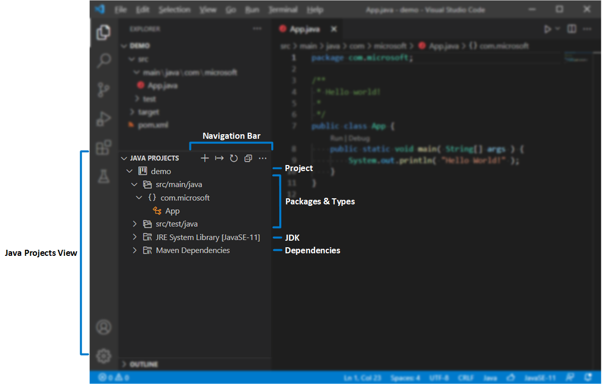
When the "Configure Classpath" window opens, click on the "Libraries" tab.
Click on "Add Library..." and select the renderer_1.jar file to add it
to the VS Code classpath.
After you add renderer_1.jar to VS Code's classpath, go back to the
ThreeDimensionalScene_R1.java file. All the little red squiggly lines
should be gone and you should be able to build and run the program.
The actions that you just took with the VS Code GUI had the effect of
creating a new subfolder and a new configuration file in the jar-example
folder. Open the jar-example folder and you should now see a new sub-folder
called .vscode that contains a new file called settings.json.
    \---jar-example
        |   renderer_1.jar
        |   ThreeDimensionalScene_R1.java
        |
        \---.vscode
                settings.json
The settings.json file holds the new classpath information for VS Code.
Here is what settings.json should look like.
{
   "java.project.sourcePaths": [
      "."
   ],
   "java.project.referencedLibraries": [
      "renderer_1.jar",
   ]
}
You can actually bypass the GUI configuration steps and just create this
folder and config file yourself. Many experienced VS Code users directly
edit their settings.json file, using, of course, VS Code. Try it. Use
VS Code to look for, and open, the settings.json file.
Now do another experiment. In VS Code, go back to the ThreeDimensionalScene_R1.java
file and hover your mouse, for several seconds, over the setColor() method
name in line 37. You should get what Microsoft calls an IntelliSense tool tip
giving you information about that method (taken from the method's Javadoc).
But the tool tips do not (yet) work for the renderer's classes. The VS Code
editor does not (yet) have the Javadoc information it needs about the
renderer's classes.
The build_jar_files.cmd script file created a second jar file called
renderer_1-sources.jar. This jar file holds all the source files from the
renderer project. This jar file can be used by VS Code to give you its
IntelliSense tool-tip information and code completion for all the renderer
classes.
Copy the file renderer_1-sources.jar from the renderer_1 folder to the
jar-example folder.
    \---jar-example
        |   renderer_1-sources.jar
        |   renderer_1.jar
        |   ThreeDimensionalScene_R1.java
        |
        \---.vscode
                settings.json
You may need to quit and restart VS Code, but VS Code should now be able to give you Javadoc tool tips when you hover your mouse (for several seconds) over any method from the renderer's classes.
NOTE: You usually do not need to explicitly add the renderer_1-sources.jar
file to the VS Code classpath. If you have added a jar file to VS Code, say
foo.jar, then VS Code is supposed to also automatically open a jar file
called foo-sources.jar if it is in the same folder as foo.jar.
FINAL NOTE: DO all the experiments mentioned in the last two sections. The experience of doing all these steps and having to figure out what you are doing wrong is far more valuable than you might think!
https://code.visualstudio.com/docs/java/java-project
https://code.visualstudio.com/docs/java/java-project#_configure-classpath-for-unmanaged-folders
If you are on the PNW campus, then you can download the following book about VS Code (you have permission to download the book, for free, while on campus because of the PNW library).
https://link.springer.com/book/10.1007/978-1-4842-9484-0
3.7 Build system summary
Every programming language needs to provide tools for working on large projects (sometimes referred to as "programming in the large").
A language should provide us with
- a system for organizing our code,
- a system for documenting our code,
- a system for building our code's artifacts,
- a system for distributing those artifacts.
For this Java renderer project we use
- classes and packages,
- Javadocs, Readmes,
- command-line scripts,
- jar files, zip files.
When you learn a new programming language, eventually you get to the stage where you need to learn the language's tools for supporting programming in the large. Learn to think in terms of how you would organize, document, build, and distribute a project.
https://en.wikipedia.org/wiki/Programming_in_the_large_and_programming_in_the_small
https://mitcommlab.mit.edu/broad/commkit/best-practices-for-coding-organization-and-documentation/
4. FrameBuffer data structure
The FrameBuffer class represents the output from our renderer.
We will consider FrameBuffer to be an abstract data type (ADT)
that has a public interface and a private implementation.
The public interface, also referred to as the class's API, defines how a
programmer works with the data type. What are its constructors and what
methods does it make available to the programmer? The public interface
to the FrameBuffer class is documented in its Javadocs. Be sure to build
and read the Javadocs for the framebuffer package.
The private implementation is the details of the class as defined in the
FrameBuffer.java source file. When you first learn about a new class,
you almost never need to know the details of its private implementation.
After you become comfortable working with the class's API, then you might
be interested in looking at its implementation. If you need to maintain or
modify a class, then you must become familiar with its implementation (its
source code).
https://en.wikipedia.org/wiki/Abstract_data_type
https://en.wikipedia.org/wiki/API
4.1 FrameBuffer interface
A FrameBuffer represents a two-dimensional array of pixel data that
can be displayed on a computer's screen as an image (a picture).
The public interface that the FrameBuffer class presents to its clients
is a two-dimensional array of colored pixels. A FrameBuffer constructor
has two parameters, widthFB and heightFB, that determine the dimensions
of the array of pixels (once a FrameBuffer is constructed, its dimensions
are immutable).
A FrameBuffer defines a two-dimensional coordinate system for its pixels.
The pixel coordinates are written like the (x, y) coordinates in a plane.
The pixel with coordinates (0, 0) is the pixel in the upper left-hand
corner. We call this pixel the "origin" of the coordinate system. The
x-coordinates increase to the right and the y-coordinates increase
downwards (there are no valid negative coordinates).
The FrameBuffer class has methods setPixelFB() and getPixelFB() for
setting and getting the color of any pixel in a FrameBuffer object. There
are also methods for storing a FrameBuffer object as an image file in the
computer's file system.
Here is a picture of a h-by-w FrameBuffer with h = 6 and w = 12.
Notice that the pixel in the upper left-hand corner of the FrameBuffer
has coordinates (0, 0) (the origin). The pixel with coordinates
(x, y) = (6, 2) is marked in the picture. That pixel is in the seventh
column and the third row (from the top). The pixel in the lower right-hand
corner has coordinates (x, y) = (w-1, h-1) = (11, 5).
       0   1  2  3  4  5  6  7  8  9 10 11
      +--+--+--+--+--+--+--+--+--+--+--+--+
    0 |  |  |  |  |  |  |  |  |  |  |  |  |
      +--+--+--+--+--+--+--+--+--+--+--+--+
    1 |  |  |  |  |  |  |  |  |  |  |  |  |
      +--+--+--+--+--+--+--+--+--+--+--+--+
    2 |  |  |  |  |  |  |##|  |  |  |  |  |
      +--+--+--+--+--+--+--+--+--+--+--+--+
    3 |  |  |  |  |  |  |  |  |  |  |  |  |
      +--+--+--+--+--+--+--+--+--+--+--+--+
    4 |  |  |  |  |  |  |  |  |  |  |  |  |
      +--+--+--+--+--+--+--+--+--+--+--+--+
    5 |  |  |  |  |  |  |  |  |  |  |  |  |
      +--+--+--+--+--+--+--+--+--+--+--+--+
Each pixel in a FrameBuffer represents the color of a single "dot" in
a computer's display screen. Most computer displays have around 1,000
horizontal pixels and 1,000 vertical pixels. The "resolution" of computer
displays varies a lot. You should find out the resolution of the display
that you are currently looking at.
We are going to take the view that Color is another abstract data type
(with a public interface and a private implementation). The Color class
is defined for us by the Java class library (in the java.awt package).
A Color object has three components, the amount of red, green, and blue
that is mixed into the color represented by the Color object.
There is much more to the FrameBuffer interface. Build and read the
Javadocs for the FrameBuffer class so that you can see the whole interface
documented in one place. (Use the script file build_all_Javadocs.cmd
to create the html folder that holds the renderer's Javadocs. Use your
browser to open the file html/index.html and then navigate to the Javadoc
page for the FrameBuffer class.)
Then, even more importantly, read the example code in the
renderer_1/clients_r1
folder and the
framebuffer-viewport-pixel-examples
sub folder. Build and run the example programs. Try making simple changes to
the example programs. Come up with your own examples of things that you
can do with a FrameBuffer.
https://en.wikipedia.org/wiki/Framebuffer
https://en.wikipedia.org/wiki/Pixel
https://en.wikipedia.org/wiki/Display_resolution
https://docs.oracle.com/en/java/javase/21/docs/api/java.desktop/java/awt/Color.html
4.2 FrameBuffer implementation
When you use an abstract data type, you normally don't need to know the
details of its (private) implementation. But since our goal is to write
the implementation of a renderer, we need to determine the details of our
implementation of the FrameBuffer interface. Since a FrameBuffer appears
to its clients to be a two-dimensional array of colors, you might expect
the FrameBuffer class to be implemented as a two-dimensional array of
Color objects, Color[][]. But that would not be a good implementation.
We shall implement the FrameBuffer class as a one-dimensional array of
integers, int[]. This array is called the pixel_buffer.
Remember that a Color object has three components, the amount of red,
green, and blue that make up the color. The human eye can see several
hundred shades of each primary color, red, green, and blue. Since our
eyes see several hundred shades of red, it is convenient to use 8 bits
(256 distinct values) to represent shades of red. Similarly for shades
of green and blue. So we need 24 bits to represent a shade of color
(notice that there are 256^3 = 2^24 = 16,777,216 distinct color shades).
A Java int is 32 bits, so we can fit the three bytes of red, green, and
blue data into a single int (and have 8 bits left over for later use).
A Java int is much more compact (in the computer's memory) that a Java
Color object. That is one reason why our FrameBuffer implementation
will use an array of (primitive) int instead of the more obvious array
of Color objects.
If a FrameBuffer represents h rows by w columns of pixels, then the
FrameBuffer's pixel_buffer holds h * w integers. Our implementation of
the FameBuffer interface does NOT store its pixel data as a two-dimensional
h-by-w array of integers (nor is it stored as a three-dimensional h-by-w-by-3
array of bytes). Our implementation of the FrameBuffer interface will store
its pixel data as a one-dimensional h * w array of integers. This
one-dimensional array is the row major form of the two-dimensional data,
meaning that the first w integers in the one-dimensional array are the
pixels from the framebuffer's first row. The next w integers in the array
are the pixels from the framebuffer's second row, etc. The first w
integers (the first row of pixels) represent the top row of pixels when
the framebuffer's image is displayed on a computer's screen.
https://en.wikipedia.org/wiki/Row-_and_column-major_order
Here is a picture of a very small h-by-w FrameBuffer (with h = 4 and
w = 7) and its array-of-rows pixel_buffer below it. Four rows and
seven columns means there are 28 pixels.
       0   1  2  3  4  5  6
      +--+--+--+--+--+--+--+
    0 |  |  |  |  |  |  |  |
      +--+--+--+--+--+--+--+
    1 |  |  |  |  |  |  |  |
      +--+--+--+--+--+--+--+
    2 |  |  |  |##|  |  |  |
      +--+--+--+--+--+--+--+
    3 |  |  |  |  |  |  |  |
      +--+--+--+--+--+--+--+


      |       row 0        |       row 1        |       row 2        |       row 3        |
      +--+--+--+--+--+--+--+--+--+--+--+--+--+--+--+--+--+--+--+--+--+--+--+--+--+--+--+--+
      |  |  |  |  |  |  |  |  |  |  |  |  |  |  |  |  |  |##|  |  |  |  |  |  |  |  |  |  |
      +--+--+--+--+--+--+--+--+--+--+--+--+--+--+--+--+--+--+--+--+--+--+--+--+--+--+--+--+
       0  1  2  3  4  5  6  7  8  9  10 11 12 13 14 15 16 17 18 19 20 21 22 23 24 25 26 27
Let us see how we would translate a two-dimensional pixel address, (x, y),
into a one-dimensional index in the pixel_buffer. Consider the pixel at
(3, 2) (column 3 and row 2) which is marked in the above picture. In the
one-dimensional pixel_buffer array, this pixel needs to skip over two whole
rows (of 7 pixels each) and then skip over three more pixels. So the index
of this pixel is 2 * 7 + 3 = 17. In general, in a FrameBuffer with width w,
a pixel at address (x, y) needs to skip over y rows (of w pixels each)
and then skip over an additional x pixels, so the pixel has an index in the
one-dimensional pixle_buffer given by
index = (y * w) + x
This formula is used by both the setPixelFB() and getPixelFB()methods
in the FrameBuffer class.
To get a better idea of how the FrameBufferinterface is implemented, let us
look at a very bare bones, minimal implementation of the FrameBuffer class.
The following FrameBuffer definition allows us to instantiate a FrameBuffer
object, read and write pixel data into the object, and print a string
representation of the object. The string representation is formatted to show
the FrameBuffer as rows of r, g, b values. This works fine for small
framebuffers (less than 20 rows by 20 columns).
import java.awt.Color;

class FrameBuffer {
   public final int width;   // Instance variables.
   public final int height;
   public final int[] pixel_buffer;

   public FrameBuffer(int width, int height) {
      this.width = width;
      this.height = height;
      this.pixel_buffer = new int[this.width * this.height];
   }

   public void setPixelFB(int x, int y, Color c) {
      pixel_buffer[(y * width) + x] = c.getRGB();
   }

   public Color getPixelFB(int x, int y) {
      return new Color( pixel_buffer[(y * width) + x] );
   }

   @Override public String toString() {
      String result = "FrameBuffer [w=" + width + ", h=" + height + "]\n";
      for (int y = 0; y < width; ++y) { result += " r   g   b |"; }
      result += "\n";
      for (int y = 0; y < height; ++y) {
         for (int x = 0; x < width; ++x) {
            final int c = pixel_buffer[(y * width) + x];
            final Color color = new Color(c);
            result += String.format("%3d ", color.getRed())
                    + String.format("%3d ", color.getGreen())
                    + String.format("%3d|", color.getBlue());
         }
         result += "\n";
      }
      return result;
   }
}
Notice that the setPixelFB() and getPixelFB() methods take two coordinate
parameters, an x and a y. The setPixelFB() method also takes a Color
parameter, and the getPixelFB() method returns a Color object. These
two methods represent the FrameBuffer as a 2-dimensional array of Color
objects (the public interface). But the data for the FrameBuffer is
stored in a 1-dimensional array of int (the private implementation).
The getPixelFB() and setPixelFB() methods do the translation from two
dimensions to one dimension, and the translation of a Color object to
an int value. (In other words, setPixelFB() translates from the public
interface to the private implementation, and getPixelFB() translates
from the private implementation to the public interface.)
Here is a sample program that creates a (small) FrameBuffer and draws
two diagonal lines in it. The program then prints the string representation
of the FrameBuffer object.
import java.awt.Color;
import java.util.Arrays;

public class TestFrameBuffer {
   public static void main(String[] args) {
      final FrameBuffer fb = new FrameBuffer(11, 11);
      for (int y = 0; y < fb.height; ++y)
         for (int x = 0; x < fb.width; ++x) {
            fb.setPixelFB(x, x, Color.white);
            fb.setPixelFB(fb.width - 1 - x, x, Color.white);
         }
      System.out.println( fb );
    //System.out.println( Arrays.toString(fb.pixel_buffer) );
   }
}
Here is what the string representation looks like after the two
diagonal lines are drawn in the FrameBuffer. Notice that this
string represents the FrameBuffer in a way that matches it public
interface (a two-dimensional array of colors). We could also print
out the pixel_buffer array from the FrameBuffer object (the
private implementation) but it is not very helpful.
FrameBuffer [w=11, h=11]
 r   g   b | r   g   b | r   g   b | r   g   b | r   g   b | r   g   b | r   g   b | r   g   b | r   g   b | r   g   b | r   g   b |
255 255 255|  0   0   0|  0   0   0|  0   0   0|  0   0   0|  0   0   0|  0   0   0|  0   0   0|  0   0   0|  0   0   0|255 255 255|
  0   0   0|255 255 255|  0   0   0|  0   0   0|  0   0   0|  0   0   0|  0   0   0|  0   0   0|  0   0   0|255 255 255|  0   0   0|
  0   0   0|  0   0   0|255 255 255|  0   0   0|  0   0   0|  0   0   0|  0   0   0|  0   0   0|255 255 255|  0   0   0|  0   0   0|
  0   0   0|  0   0   0|  0   0   0|255 255 255|  0   0   0|  0   0   0|  0   0   0|255 255 255|  0   0   0|  0   0   0|  0   0   0|
  0   0   0|  0   0   0|  0   0   0|  0   0   0|255 255 255|  0   0   0|255 255 255|  0   0   0|  0   0   0|  0   0   0|  0   0   0|
  0   0   0|  0   0   0|  0   0   0|  0   0   0|  0   0   0|255 255 255|  0   0   0|  0   0   0|  0   0   0|  0   0   0|  0   0   0|
  0   0   0|  0   0   0|  0   0   0|  0   0   0|255 255 255|  0   0   0|255 255 255|  0   0   0|  0   0   0|  0   0   0|  0   0   0|
  0   0   0|  0   0   0|  0   0   0|255 255 255|  0   0   0|  0   0   0|  0   0   0|255 255 255|  0   0   0|  0   0   0|  0   0   0|
  0   0   0|  0   0   0|255 255 255|  0   0   0|  0   0   0|  0   0   0|  0   0   0|  0   0   0|255 255 255|  0   0   0|  0   0   0|
  0   0   0|255 255 255|  0   0   0|  0   0   0|  0   0   0|  0   0   0|  0   0   0|  0   0   0|  0   0   0|255 255 255|  0   0   0|
255 255 255|  0   0   0|  0   0   0|  0   0   0|  0   0   0|  0   0   0|  0   0   0|  0   0   0|  0   0   0|  0   0   0|255 255 255|
The last two class definitions, for FrameBuffer and TestFrameBuffer,
are compilable and runnable. Try running these examples and make sure
you get the output shown above. Also, try modifying and experimenting
with these examples.
4.3 FrameBuffer objects and PPM files
An instance of the FrameBuffer class is a data structure (a Java object).
It "lives" inside the computer's memory system (in the Java heap). We cannot
see a FrameBuffer object (but we can "visualize" it using its toString()
method). But the whole point of computer graphics is to see the 3D images the
renderer can create. So how do we actually see the image that a FrameBufffer
object represents?
We need to copy the data from a FrameBuffer object into an image file in
the computer's file system (that is, we need to copy data from the computer's
memory system to the computer's file system). When you take a picture with a
digital camera, the picture ends up as an image file in the camera's storage
device. You can "open" that image file and see the picture it represents
displayed on a screen. You can send that image file to someone else's
computer and then they can see the image displayed on their screen. Image
files are how we preserve the data from a FrameBuffer object.
An image file format is a specific way to store pixel data in a file. There are a large number of image file formats. Most of the well known ones (png, jpeg, heic) are more complicated than what we need. We will use a simple image file format that is popular with programmers who experiment with 3D renderers, the PPM file format.
A PPM file has two parts, the meta-data part and the pixel-data part. The meta-data part is data about the pixel-data part. Before we can explain the meta-data part, we need to explain the pixel-data part.
The pixel-data in a PPM file is a sequence of (binary) bytes, three bytes for every pixel in the image represented by the PPM file. If a PPM file represents an image that is 300 pixels wide and 200 pixels tall, then there are 60,000 pixels in the image and 180,000 bytes in the pixel-data part of the PPM file. The first three bytes in the pixel-data are the bytes for the first pixel in the image (the upper left-hand corner of the image). The three bytes for each pixel are in the order red, green, blue.
We just said that an image that is 300 pixels wide and 200 pixels tall will have 180,000 bytes of pixel-data. But suppose you are presented with 180,000 bytes of pixel-data. How wide is the image? How tall is the image? Maybe it is 300 pixels wide and 200 pixels tall, but maybe it is 200 pixels wide and 300 pixels tall. Or maybe the image represented by this pixel-data is 400 pixels wide and 150 pixels tall (or 150 pixels wide and 400 pixels tall). All of the following image dimensions have the same number of bytes of pixel-data.
- 300 by 200
- 200 by 300
- 100 by 600
- 400 by 150
- 800 by 75
The pixel-data in a PPM file is ambiguous. By itself it cannot tell us what the dimensions are of the image it represents. So we need more information about the pixel-data. That is the "meta data" (data about data). The first part of a PPM file, the meta-data part, tells us the dimensions of the image represented by the pixel-data.
A PPM file begins with three lines of ASCII text. The first line is called the "magic number" and it should contain the string "P6". The second line contains the dimensions of the image and should put the width first, followed by a space, and then the height. The third line should contain the string "255" to specify that we are using 255 values for each of red, green, and blue (i.e., one byte).
The meta-data (also called the "file header") for the PPM file of an image that is 300 pixels wide and 200 pixels tall would be,
P6
300 200
255
and then this meta-data would be immediately followed in the file by the 180,000 bytes of pixel-data.
One somewhat odd characteristic of a P6 PPM file is that it is both a "text file" and a "binary file". The first part of the PPM file, the meta-data, is ASCII text. But the second part of the PPM file, the pixel-data, is binary data. You should open a PPM file in a text editor and notice that the meta-data is clearly readable, but where the meta-data ends, the file becomes "unreadable".
The FrameBuffer class has methods for saving a FrameBuffer object as a PPM
file. The FrameBuffer class also has a constructor for creating a FrameBuffer
object initialized with the pixel data from a PPM file. See the FrameBuffer
Javadocs for details.
https://en.wikipedia.org/wiki/Netpbm#File_formats
https://en.wikipedia.org/wiki/Image_file_format
https://developer.mozilla.org/en-US/docs/Web/Media/Guides/Formats/Image_types
https://en.wikipedia.org/wiki/Metadata
5. Viewport data structure
The Viewport class represents a rectangular region of pixels in a
FrameBuffer. We will consider Viewport to be another abstract data
type with a public interface and a private implementation.
Be sure to build the Javadocs for the framebuffer package and look at
the Javadocs for the Viewport class (its public interface).
After you become familiar with the Viewport interface from the Javadocs
and the code examples, then you can look at the source code for the
Viewport class to learn the details of its implementation.
5.1 Viewport interface
The FrameBuffer class defines a nested Viewport class which represents
a rectangular sub-array of the pixel data in the FrameBuffer. A Viewport
is the active part of the FrameBuffer; it is the part of the FrameBuffer
that the renderer writes pixel data into.
The Viewport interface is similar to theFrameBuffer` interface.
A Viewport is determined by its width and height and the position of its
upper left-hand corner in the FrameBuffer. A Viewport constructor has
four parameters, widthVP, heightVP. ul_x and ul_y. In order that a
Viewport be completely contained in its Framebuffer, we should have
    ul_x +  widthVP <  widthFB   and
    ul_y + heightVP < heightFB
where widthFB and heightFB are the width and the height of the
FrameBuffer.
Each Viewport has its own (x,y)-coordinate system for the pixels within
the Viewport. This coordinate system has its origin, (0,0), at the upper
left-hand corner of the Viewport. The x-coordinates increase to the right
and the y-coordinates increase downwards.
The Viewport class has methods setPixelVP() and getPixelVP()for setting
and getting the color of any pixel in a Viewport. There are also methods
for storing a Viewport as an image file in the computer's file system.
Here is an illustration of a FrameBuffer that has n rows by m columns
of pixels with a Viewport that has w rows and h columns. Notice how,
in this picture, the upper left-hand corner of the Viewport is labeled
(0,0). This is that pixel's coordinate in the Viewport's coordinate
system. In the coordinate system of the FrameBuffer that pixel has the
coordinate (x_ul, y_ul).
      (0,0)
        +-------------------------------------------+
        |                                           |
        |                                           |
        |        (0,0)                              |
        |          +------------+                   |
        |          |            |                   |
        |          |            |                   |
        |          |            |                   |
        |          |            |                   |
        |          +------------+                   |
        |                   (w-1,h-1)               |
        |                                           |
        |                                           |
        |                                           |
        |                                           |
        +-------------------------------------------+
                                                (m-1,n-1)
Quite often a Viewport will be the whole FrameBuffer. A Viewport
that is smaller than the whole FrameBuffer can be used to implement
special effects like "split screen" (two independent images in the
FrameBuffer), or "picture in a picture" (a smaller picture superimposed
on a larger picture). In future renderers (starting with renderer 5),
another use of a Viewport that is not the whole FrameBuffer is when we
want to display an image with an aspect ratio that is different than the
aspect ratio of the FrameBuffer.
https://en.wikipedia.org/wiki/Split_screen_(computer_graphics)
https://en.wikipedia.org/wiki/Picture-in-picture
5.2 Viewport implementation
The Viewport class is implemented as a non-static nested class
(also called an inner class) within the FrameBuffer class. Inner
classes are not always covered in introductory Java textbooks but
they are fairly common in the design of larger software systems.
https://docs.oracle.com/javase/tutorial/java/javaOO/nested.html
https://dev.java/learn/classes-objects/nested-classes/
https://www.baeldung.com/java-nested-classes
A nested class (inner class) is a class defined inside the definition
of some other class (the outer class). Here is a (very) brief outline
of the FrameBufer class and its inner Viewport class.
import java.awt.Color;

class FrameBuffer
{
   final int widthFB;   // Instance variables.
   final int heightFB;
   final int[] pixel_buffer;

   public FrameBuffer(int widthFB, int heightFB)
   {
      this.widthFB = widthFB;
      this.heightFB = heightFB;
      this.pixel_buffer = new int[widthFB * heightFB];
   }

   public void setPixelFB(int x, int y, Color c)
   {
      pixel_buffer[(y * widthFB) + x] = c.getRGB();
   }

   public Color getPixelFB(int x, int y)
   {
      return new Color( pixel_buffer[(y * widthFB) + x] );
   }

   public class Viewport // Inner class.
   {
      final int vp_ul_x; // Instance variables for inner class.
      final int vp_ul_y;
      final int widthVP;
      final int heightVP;
      public Viewport(int ul_x, int ul_y, int widthVP, int heightVP)
      {
         this.vp_ul_x = ul_x;
         this.vp_ul_y = ul_y;
         this.widthVP = widthVP;
         this.heightVP = heightVP;
      }
      public void setPixelVP(int x, int y, Color c)
      {
         setPixelFB(vp_ul_x + x, vp_ul_y + y, c);
      }
      public Color getPixelVP(int x, int y)
      {
         return getPixelFB(vp_ul_x + x, vp_ul_y + y);
      }
   }
}
A nested class is defined in a way that is similar to how methods are
defined. A method is nested within a class definition and a method has
access to all the fields and other methods defined in the class. The same
is true for a nested class; it has access to all the fields and methods
defined in its outer class. But this is a very subtle idea. In order that
a nested class have access to the instance fields of its outer class, the
nested class must be instantiated with respect to a specific instance of
the outer class. In other words, an instance of the inner class cannot
have access to the fields of every and any instance of the outer class.
It would only make sense for an instance of the inner class to have access
to the fields of a specific instance of the outer class. For example, here
is the code for instantiating a FrameBuffer object and an associated
Viewport object.
    final FrameBuffer fb = new FrameBuffer(100, 100);

    final FrameBuffer.Viewport vp = fb.new Viewport(20, 20, 50, 50);
The FrameBuffer.Viewport notation is because the ViewPort class is a member
class of the FrameBuffer class. The fb.new notation is what specifies that
the new instance of the Viewport class must be tied to the fb instance of
FrameBuffer.
Notice that there is no pixel-array in the definition of the Viewport
class. A Viewport object does not store any pixel data. Instead of pixel
data, a Viewport object has a (hidden) reference to its FrameBuffer object.
The Viewport object vp has access to all the fields and methods of the
FrameBuufer object fb (using vp's hidden reference to fb). In particular,
a Viewport has access to the pixel_buffer of the FrameBuffer. A Viewport
object gets all of its pixel data from the FrameBuffer object it is tied
to. When you access a pixel within a Viewport object, using either the
getPixelVP() or setPixleVP() methods, you are really accessing a pixel
in the FrameBuffer object that owns that Viewport object.
Here is an illustration of a FrameBuffer containing two Viewports and
another FrameBuffer containing a single Viewport.
      fb1
    +------------------------------------------+
    |                                          |         fb2
    |     +------------+                       |       +-----------------------------+
    |     |            |                       |       |                             |
    |     |            |                       |       |     +------------+          |
    |     |            |                       |       |     |            |          |
    |     |            |                       |       |     |            |          |
    |     +------------+                       |       |     |            |          |
    |                                          |       |     |            |          |
    |                       +------------+     |       |     +------------+          |
    |                       |            |     |       |                             |
    |                       |            |     |       |                             |
    |                       |            |     |       +-----------------------------+
    |                       |            |     |
    |                       +------------+     |
    +------------------------------------------+
Here is code that can instantiates these five objects.
    final FrameBuffer fb1 = new FrameBuffer(300, 250);
    final FrameBuffer fb2 = new FrameBuffer(200, 150);
    final FrameBuffer.Viewport vp1 = fb1.new Viewport( 30,  30, 100, 100);
    final FrameBuffer.Viewport vp2 = fb1.new Viewport(150, 150,  75,  75);
    final FrameBuffer.Viewport vp3 = fb2.new Viewport( 30,  30,  80,  80);
Remember that the fb1.new and fb2.new notation reminds us that each
instance of the Viewport class must be tied to a specific instance
of the FrameBuffer class.
After executing these five lines of code, the Java heap will contain five
objects, two FrameBuffer objects and three ViewPort objects. Each
Viewport object is "tied" to a specific FrameBuffer object (using a
hidden reference variable in the Viewport object). A Viewport does
not itself store any pixel data. Each Viewport object references its
FrameBuffer object to access the pixels that are represented by the
Viewport.
Let us look more carefully at an example of a FrameBuffer containing a
Viewport. Here is code that instantiates a (small) FrameBuffer that
has 5 rows and 8 columns of pixels with a (even smaller) Viewport that
has 3 rows and 4 columns, and with the Viewport's upper left-hand corner
at pixel (2, 1) in the FrameBuffer.
   final FrameBuffer fb = new FrameBuffer(8, 5);
   final FrameBuffer.Viewport vp = fb.new Viewport(2, 1, 4, 3);
Here is a representation of this FrameBuffer and its Viewport.
       0   1  2  3  4  5  6  7
      +--+--+--+--+--+--+--+--+
    0 |  |  |  |  |  |  |  |  |
      +--+--+--+--+--+--+--+--+
    1 |  |  |##|##|##|##|  |  |
      +--+--+--+--+--+--+--+--+
    2 |  |  |##|##|##|##|  |  |
      +--+--+--+--+--+--+--+--+
    3 |  |  |##|##|##|##|  |  |
      +--+--+--+--+--+--+--+--+
    4 |  |  |  |  |  |  |  |  |
      +--+--+--+--+--+--+--+--+
Here is how the rows of the Viewport are positioned within the
FrameBuffer's one-dimensional array-of-rows pixel_buffer. Notice
that the Viewport's three rows are NOT contiguous within the
pixel_buffer.
    |         row 0         |         row 1         |         row 2         |         row 3         |         row 4         |
    +--+--+--+--+--+--+--+--+--+--+--+--+--+--+--+--+--+--+--+--+--+--+--+--+--+--+--+--+--+--+--+--+--+--+--+--+--+--+--+--+
    |  |  |  |  |  |  |  |  |  |  |##|##|##|##|  |  |  |  |##|##|##|##|  |  |  |  |##|##|##|##|  |  |  |  |  |  |  |  |  |  |
    +--+--+--+--+--+--+--+--+--+--+--+--+--+--+--+--+--+--+--+--+--+--+--+--+--+--+--+--+--+--+--+--+--+--+--+--+--+--+--+--+
     0  1  2  3  4  5  6  7  8  9  10 11 12 13 14 15 16 17 18 19 20 21 22 23 24 25 26 27 28 29 30 31 32 33 34 35 36 37 38 39
Given a Viewport pixel with coordinates (i, j)``, we know that itsFramebuffercoordinates are(x_ul + i, y_ul + j). From thoseFrameBuffercoordinates we
know that the(i, j)pixel from theViewporthas the followingindexin theFrameBuffer'spixel_buffer`.
index = (y_ul + j) * w + (x_ul + i)
For example, consider pixel (2, 1) in the Viewport.
       0   1  2  3  4  5  6  7
      +--+--+--+--+--+--+--+--+
    0 |  |  |  |  |  |  |  |  |
      +--+--+--+--+--+--+--+--+
    1 |  |  |##|##|##|##|  |  |
      +--+--+--+--+--+--+--+--+
    2 |  |  |##|##|@@|##|  |  |
      +--+--+--+--+--+--+--+--+
    3 |  |  |##|##|##|##|  |  |
      +--+--+--+--+--+--+--+--+
    4 |  |  |  |  |  |  |  |  |
      +--+--+--+--+--+--+--+--+
It is pixel (x_ul + i, y_ul + j) = (2 + 2, 1 + 1) = (4, 2) in the
FrameBuffer. That FrameBuffer pixel has the following index in the
pixel_buffer.
index = (y_ul + j) * w + (x_ul + i) = (1 + 1) * 8 + (2 + 2) = 20
    |         row 0         |         row 1         |         row 2         |         row 3         |         row 4         |
    +--+--+--+--+--+--+--+--+--+--+--+--+--+--+--+--+--+--+--+--+--+--+--+--+--+--+--+--+--+--+--+--+--+--+--+--+--+--+--+--+
    |  |  |  |  |  |  |  |  |  |  |##|##|##|##|  |  |  |  |##|##|@@|##|  |  |  |  |##|##|##|##|  |  |  |  |  |  |  |  |  |  |
    +--+--+--+--+--+--+--+--+--+--+--+--+--+--+--+--+--+--+--+--+--+--+--+--+--+--+--+--+--+--+--+--+--+--+--+--+--+--+--+--+
     0  1  2  3  4  5  6  7  8  9  10 11 12 13 14 15 16 17 18 19 20 21 22 23 24 25 26 27 28 29 30 31 32 33 34 35 36 37 38 39
5.3 Clearing a FrameBuffer or Viewport
When a FrameBuffer is created, how should its pixel data be initialized?
One possibility is to leave the FrameBuffer's pixel_buffer filled with
whatever Java's array constructor puts in it. A better strategy is to
have specific rules about initializing FrameBuffer objects.
Every FrameBuffer object has a "background color" field. If you do not
specify a FrameBuffer's background color when constructing the FrameBuffer,
the color defaults to black. When a FrameBuffer object is constructed, all
of its pixel data is initialized to the FrameBuffer's background color.
The FrameBuffer class has a clearFB() method that resets all the pixel
data in the FrameBuffer object to the background color. This "erases"
the FrameBuffer.
Every Viewport object also has a "background color" but the rules for
a Viewport are a bit different. When a Viewport is created, its
pixels are not set to its background color. The idea is that creating a
Viewport should not destroy (erase) the pixel data it represents in
the FrameBuffer.
The Viewport class has a clearVP() method that resets all the pixels
represented by the Viewport object to the background color of the
Viewport'. This erases theViewport, which will also erase the part
of theFrameBufferrepresent by theViewport`.
Here are a few rules that summarize the interactions between the FrameBuffer
background color and the background color for any Viewport.
- The default background color for a
FrameBufferis black. - When a new
FrameBufferis created, it is cleared with its background color. - Resetting the background color of a
FrameBuffer' does not clear theFrameBuffer. - The default background color for a
Viewportis the background color of its parentFrameBuffer. - When a new
Viewportis created, it is NOT cleared (so you can copy, or modify, whatever pixels are in that region of theFrameBuffer). - Resetting the background color of a
Viewportdoes not clear theViewport. - Resetting background color of a
FrameBufferdoes not reset the background color of anyViewport, not even the defaultViewport. - Clearing a
FrameBufferwill also clear all itsViewports to the background color of theFrameBuffer.
If you want to see more examples of code that uses the FrameBuffer and
Viewport classes, look at the code in the follow zip file.
http://cs.pnw.edu/~rlkraft/cs45500/for-class/framebuffer-viewport-pixel-examples.zip
6. Scene data structure
A Scene data structure represents a collection of geometric shapes
positioned in three dimensional space.
Here are the data field declarations from the Scene class.
public final class Scene
{
   public final Camera camera;
   public final List<Position> positionList;
   public final String name;

}
A Scene object holds a reference to a Camera object and a reference
to a List of Position objects. A Scene object also holds a reference
to a String that gives the scene a "name". This name is mainly for debugging
and documentation purposes.
Each Position object holds a Model object (which represents a geometric
shape, see below) and a Vector object (which represents a location in
3D camera space). Each Model is positioned, by its Vector, in front of
the Camera which is located at the origin and looks down the negative
z-axis. Each Model object in a Scene object represents a distinct
geometric shape in the scene. A Model object is a List of Vertex
objects and a List of Primitive objects. A Primitive is either a
LineSegment or a Point. Each LineSegment object refers to two of
the Model's Vertex objects. The Vertex objects represent points in
the model's own coordinate system. The model's line segments represent
the geometric object as a "wire-frame", that is, the geometric object
is drawn as a collection of "edges". This is a fairly simplistic way
of doing 3D graphics and we will improve this in later renderers.
https://en.wikipedia.org/wiki/Wire-frame_model
https://www.google.com/search?q=3d+graphics+wireframe&tbm=isch
7. Camera
A Camera object represents a camera located at the origin of 3-dimensional
space looking down the negative z-axis. The 3-dimensional space looks like
this.
                      y-axis
                       |
                     2 +              -z-axis
                       |               /
                       |              /
                       |          -2 +
                       |      |     /
                       |      |    /     This 3D space is called "camera space".
                       |      |   /
                       |      |  /
                     1 +      | /
                       |      |/
                       |   -1 +------------ z = -1 is the Camera's "image-plane"
                       |     /
                       |    /
                       |   /
                       |  /
                       | /
                Camera |/
    --+----------------+----------------+---------> x-axis
     -1               /0                1
                     / |
                    /  |
                   /
                z-axis
We call this 3-dimensional space camera space. The xy-plane of camera space is parallel to the computer screen. The positive x-axis extends to the right on the computer's screen and the positive y-axis extends upwards. The negative z-axis extends into the computer screen and the positive z-axis extends out of the computer screen. Since the camera is at the origin and is "looking" down the z-axis in the negative direction, the camera cannot "see" anything that is positioned with a positive z-coordinate.
A Camera object has associated to it a view volume that determines what
part of camera space the camera can "see" when we use the camera to take
a picture (that is, when we render a Scene object). The camera "sees"
any geometric shape (Model object) that is positioned within its view
volume. Any geometry that is outside of the camera's view volume is
invisible to the camera.
A camera can "take a picture" two ways, using a "perspective projection" or a "parallel projection" (also called an "orthographic projection"). Each way of taking a picture has a different shape for its view volume.
For the perspective projection, the view volume is an infinitely long pyramid that is formed by the pyramid with its apex at the origin and its base in the plane z = -1 with edges x = -1, x = +1, y = -1, and y = +1.

https://webglfundamentals.org/webgl/frustum-diagram.html
https://cs.wellesley.edu/~cs307/threejs/demos-s21-r95/Camera/frustum.shtml
https://cs.wellesley.edu/~cs307/threejs/demos-s21-r95/Camera/camera-api.shtml
For the orthographic projection, the view volume is an infinitely long
rectangular cylinder parallel to the z-axis and with sides x = -1,
x = +1, y = -1, and y = +1 (an infinite parallelepiped).

https://webglfundamentals.org/webgl/webgl-visualize-camera-with-orthographic.html
When the graphics rendering pipeline uses a Camera to render a Scene,
the renderer "sees" only the geometry from the Scene that is contained
in the camera's view volume. Notice that this means the orthographic camera
will see geometry that is behind the camera. (In fact, the perspective camera
also sees geometry that is behind the camera because its view frustum is
really double ended.) The renderer's Rasterize pipeline stage is responsible
for making sure that the scene's geometry that is outside of the camera's view
volume is not visible. Any geometry outside of the view volume will be "clipped"
off.
The plane z = -1 is called the camera's image-plane. The rectangle in
the image-plane with corners (-1, -1, -1) and (+1, +1, -1) is called the
camera's view rectangle.
               View Rectangle
       (in the Camera's image-plane, z = -1)

                   y-axis
                     |
                     |     (+1,+1,-1)
          +---------------------+
          |          |          |
          |          |          |
          |          |          |
          |          |          |
       ---|----------+----------|------ x-axis
          |          |          |
          |          |          |
          |          |          |
          |          |          |
          +---------------------+
     (-1,-1,-1)      |
                     |
The view rectangle is like the film in a real camera; it is where the
camera's image appears when you take a picture. Taking a picture means
that the models in the scene get projected flat onto the view rectangle
by the camera. The contents of the camera's view rectangle (after the
projection) is what gets rasterized, by the renderer's Rasterize
pipeline stage, into a FrameBuffer's Viewport.
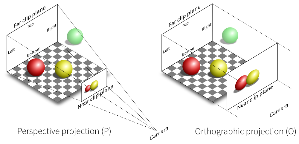
https://webglfundamentals.org/webgl/frustum-diagram.html
https://math.hws.edu/graphicsbook/demos/c3/transform-equivalence-3d.html
https://threejs.org/examples/#webgl_camera
8. Model, Vertex, Color, Primitive
A Model data structure represents a distinct geometric shape in a Scene.
Here are the data field declarations from the Model class.
public class Model
{
   public final List<Vertex>    vertexList;
   public final List<Color>     colorList;
   public final List<Primitive> primitiveList;
   public final String name;

}
A Model object contains references to a List of Vertex objects,
a List of Color objects, and a List of Primitive objects (which
are either LineSegment or Point objects). There is also a String
that is used mostly for documentation and debugging.
The Vertex objects represent points from the geometric shape that we
are modeling. Each Vertex object holds three double values that
represent the coordinates of that Vertex in three-dimensional space.
public final class Vertex
{
   public final double x, y, z;

}
In the real world, a geometric object has an infinite number of points. In 3D graphics, we "approximate" a geometric object by listing just enough points to adequately describe the shape of the object. For example, in the real world, a rectangle contains an infinite number of points, but it can be adequately modeled by just its four corner points. (Think about a circle. How many points does it take to adequately model a circle?)
If we model a rectangle by using just its four corner points, then how
do we represent the rectangle's four edges? That is what we use the
LineSegment class for.
Each LineSegment object contains two positive integers that are the
indices of two Vertex objects from the Model's vertex list. Each
of those two Vertex objects contains the xyz-coordinates for one of
the line segment's two endpoints. A LineSegment is used to represent
an edge in a geometric shape.
A LineSegment is a subclass of the Primitive class (we say that a
LineSegment "is a " Primitive). The LineSegment class does not
declare any data fields. It inherits its data fields from the
declarations in the Primitive super class.
public class LineSegment extends Primitive
{

}

public abstract class Primitive
{
   public final List<Integer> vIndexList;
   public final List<Integer> cIndexList;

}
We use LineSegment objects to "fill in" the space between a model's
vertices. For example, while a rectangle can be approximated by its four
corner points, those same four points can also represent a U shaped figure,
a Z shaped figure, or an X shaped figure.
    v3      v2         v3      v2         v3      v2         v3      v2
     +------+           +      +           +------+           +      +
     |      |           |      |                 /             \    /
     |      |           |      |                /               \  /
     |      |           |      |               /                 \/
     |      |           |      |              /                  /\
     |      |           |      |             /                  /  \
     |      |           |      |            /                  /    \
     +------+           +------+           +------+           +      +
    v0      v1         v0      v1         v0      v1         v0      v1
Given the collection of vertices in a model, we use line segments to "fill in" the space between the vertices and to outline a geometric shape for the model.
Here is a simple example. Here are four Vertex objects that represent
the four corners of a square.
    final Vertex v0 = new Vertex(0, 0, 0),
                 v1 = new Vertex(1, 0, 0),
                 v2 = new Vertex(1, 1, 0),
                 v3 = new Vertex(0, 1, 0);
Create a Model object and add those Vertex objects to the Model object.
    final Model m = new Model();
    m.addVertex(v0, v1, v2, v3);
So far the Model has four vertices in it, but we have not yet specified
how those vertices are connected to each other. The Model is not yet
ready to be rendered.
These four LineSegment objects make the Model into a square.
    m.addPrimitive(new LineSegment(0, 1),  // connect v0 to v1
                   new LineSegment(1, 2),  // connect v1 to v2
                   new LineSegment(2, 3),  // connect v3 to v3
                   new LineSegment(3, 0)); // connect v3 back to v0
On the other hand, these three LineSegment objects would make the four
vertices into a U shape.
    m.addPrimitive(new LineSegment(3, 0),  // connect v3 to v0
                   new LineSegment(0, 1),  // connect v0 to v1
                   new LineSegment(1, 2)); // connect v1 to v2
These three LineSegment objects would make the four vertices into a Z shape.
    m.addPrimitive(new LineSegment(3, 2),  // connect v3 to v2
                   new LineSegment(2, 0),  // connect v2 to v0
                   new LineSegment(0, 1)); // connect v0 to v1
These two LineSegment objects would make the four vertices into an X shape.
    m.addPrimitive(new LineSegment(0, 2),  // connect v0 to v2
                   new LineSegment(1, 3)); // connect v1 to v3
Compare these four code fragments to the four picture just above. Make sure you see how each code fragement creates the appropriate geometric shape.
If we want our Model to be just four points, with no connecting line
segments, then we can use Point primitives instead of LineSegmnt
primitives. A Point object contains an integer that is the index
of a single Vertex object from the vertex list in the Model.
    m.addPrimitive(new Point(0),   // v0 by itself
                   new Point(1),   // v1 by itself
                   new Point(2),   // v2 by itself
                   new Point(3));  // v3 by itself
Normally a Point primitive is rasterized as a single pixel but a single
pixel may barely be visible on a monitor screen. We can make a Point
primitive more visible by increasing the radius of its rasterization.
    final Point p0 = new Point(0),
                p1 = new Point(1),
                p2 = new Point(2),
                p3 = new Point(3));
    p0.radius = 2; // Make each point appear larger.
    p1.radius = 2;
    p2.radius = 2;
    p3.radius = 2;
    m.addPrimitive(p0, p1, p2, p3);
The Point class is a subclass of the Primitive class. Like the
LineSegment class, it inherits its Vertex list and Color list
from the Primitive superclass. But the Point class adds one new
data field, the rasterization radius for the point.
public class Point extends Primitive
{
   public int radius = 0;  // mutable radius

}
We can mix Point and LineSegment primitives in a Model. Since both
Point and LineSegment are of type Primitive, they can be placed
together in a model's List<Primitive>. For example, the following Model
has one diagonal line segment with a point on either side of it, similar to
a '%' symbol.
    final Model m = new Model("Percent");
    m.addPrimitive(new Point(1),           // v1 by itself.
                   new LineSegment(0, 2),  // Connect v0 to v2.
                   new Point(3));          // v3 by itself.
This would look something like following picture.
    v3      v2
     +      +
           /
          /
         /
        /
       /
      /
     +      +
    v0      v1
Exercise: Modify the code to make the two points appear larger when they get rendered.
If we model a circle using just points, we would probably need to draw
hundreds of points to get a solid looking circle with no visible gaps
between points around the circumference. But if we connect every two
adjacent points around the circumference of the circle with a short line
segment, then we can get a good model of a circle with just a few dozen
points. Look at the Circle.java class in the renderer.models_L package.
Our models represent geometric objects as a wire-frame of line segments. That is, a geometric object is drawn as a collection of "edges".
https://en.wikipedia.org/wiki/Wire-frame_model
https://www.google.com/search?q=computer+graphics+wireframe&udm=2
This is a fairly simplistic way of doing 3D graphics and we will improve this in a later renderer. Let us briefly look at how.
The current version of the renderer draws wireframe objects. Four
vertices can draw the outline of a rectangle. But what about drawing
a filled in, solid looking, rectangle? This is done by defining a new
kind of Primitive object, a Triangle.
A LineSegment primitive uses two vertices to represent a line segment.
The renderer, in its rasterization stage, "fills in" the space between the
line segment's two endpoints. Using four vertices and four line segments
we can represent the outline of a rectangle.
While two points can only be "filled in" by a one-dimensional line segment, three point can be "filled in" as a two-dimensional solid triangle.
A Triangle primitive uses three vertices from a Model. The renderer's
rasterization stage will "fill in" all the pixels in the interior of the
triangle and draw a solid triangle shape. Using four vertices and two
triangles, we can represent a solid rectangle.
    v3______________v2
      |@@@@@@@@@@/#|
      |@@@@@@@@@/##|
      |@@@@@@@@/###|
      |@@@@@@@/####|
      |@@@@@@/#####|
      |@@@@@/######|
      |@@@@/#######|
      |@@@/########|
      |@@/#########|
      |@/##########|
      +------------+
     v0            v1
Here is what the code will look like.
    final Model m = new Model("Solid_Rectangle");
    m.addVertex(new Vertex(0, 0, 0),
                new Vertex(1, 0, 0),
                new Vertex(1, 1, 0),
                new Vertex(0, 1, 0));
    m.addPrimitive(new Triangle(0, 2, 1),  // Lower right triangle.
                   new Trinagle(0, 3, 2)); // Upper left triangle.
Modern computer graphics systems combine millions of small triangles into "triangle meshes" that can represent almost any geometric shape in a game or an animation.
https://en.wikipedia.org/wiki/Polygon_triangulation
https://en.wikipedia.org/wiki/Polygon_mesh
https://www.google.com/search?q=computer+graphics+polygon+mesh&udm=2
https://en.wikipedia.org/wiki/Geometric_primitive
8.1 Vertex, Color, Primitive
We have not said much about color yet. A Model object has a List' ofColor` objects, but we have not yet explained how we make use of it.
Just as a LineSegment contains two integer values that are used as
indexes into the Model's List<Vertex>, one Vertex index for each
endpoint of the LineSgement, each LineSegment also contains another
two integer values that are used as indexes into the Model's List<Color>,
one Color index for each endpoint of the LineSegment. This allows us to
assign a color to each endpoint of a line segment.
For example, we might assign the color red to both endpoints of a line segment and we would expect this to give us a red colored line segment. Here is an illustration of how we can think about this configuration.
    List<Vertex>      List<Color>      List<Primitive>
      +------+         +------+        +---------------+
    0 |  v0  |       0 |  c0  |      0 | [0, 1] [0, 0] |  // LineSegment
      +------+         +------+        +---------------+
    1 |  v1  |
      +------+
Our List<Vertex> contain two Vertex objects. Our List<Color> contains
a single Color object. Our List<Primitive> contains a single LineSegment
object which contains two List<Integer> objects. The first List contains
two integer indices into the List<Vertex>. The second List contains two
integer indices into the List<Color>. Here is the code that creates this
configuration.
    final Model m = new Model();
    m.addVertex(new Vertex(0, 0, 0),             // v0
                new Vertex(1, 0, 0));            // v1
    m.addColor(new Color(1, 0, 0));              // c0, red
    m.addPrimitive(new LineSegment(0, 1, 0, 0)); // vertex, vertex, color, color
Notice how the LineSegment constructor is given four integer values. The
first two are indices into the vertex list and the last two are indices into
the color list. (There are other, overloaded, ways to call the LineSegment
constructor. See the Javadocs page for the LineSegment class.)
On the other hand, we might assign the color red to one endpoint of the line segment and the color blue to the other endpoint,
    final Model m = new Model();
    m.addVertex(new Vertex(0, 0, 0),             // v0
                new Vertex(1, 0, 0));            // v1
    m.addColor(new Color(1, 0, 0),               // c0, red
               new Color(0, 0, 1));              // c1, blue
    m.addPrimitive(new LineSegment(0, 1, 0, 1)); // vertex, vertex, color, color
which we can think about this way.
    List<Vertex>      List<Color>       List<Primitive>
      +------+         +------+        +---------------+
    0 |  v0  |       0 |  c0  |      0 | [0, 1] [0, 1] |  // LineSegment
      +------+         +------+        +---------------+
    1 |  v1  |       1 |  c1  |
      +------+         +------+
What color does that make the line segment? We would expect the color of
the line segment to gradually shift from c0 on one end to c1 on the
other end with shades varying from c0 to c1 in between. The shades
between c0 and c1 are called interpolated colors.
8.2 Interpolated Color
Suppose that the v0 end of the line segment is red and the v1 end is
blue. We want the color of the line segment to gradually shift from red to
blue as our position on the line segment shifts from v0 to v1. At the
half way point between vo and v1 we should see the color purple, which
is half way between red and blue. Since red has
(r, g, b) = (1.0, 0.0, 0.0), // red
and blue has
(r, g, b) = (0.0, 0.0, 1.0), // blue
half way between red and blue we should see a color whose red component is half way between 1.0 and 0.0, or 0.5, and whose blue component is half way between 0.0 and 1.0, also 0.5 (and whose green component is half way between 0.0 and 0.0, or 0.0). So the color in the middle of the line segment should be an equal mix of red and blue, a shade of purple.
(r, g, b) = (0.5, 0.0, 0.5), // purple
We can write a formula for the interpolated color along a line segment.
The line segment between v0 and v1 can be described by the following
vector parametric equation (also called the lerp formula).
p(t) = (1 - t)*v0 + t*v1 with 0.0 <= t <= 1.0
We think of the variable t as representing time and p(t) representing
a point moving along the line from time t=0 to time t=1. At time 0,
we start at v0,
p(0) = (1 - 0)*v0 + 0*v1 = v0
while at time 1 we end up at v1,
p(1) = (1 - 1)*v0 + 1*v1 = v1.
We can also think of the lerp formula as saying that p(t) is a weighted
average of v0 and v1, with weights 1-t and t. When t=0, all the
weight is on p0. When t=1, all the weight is on v1. When t=1/2,
half the weight is on each point, and we should be at the point midway
between them.
Let v0 = (x0, y0, z0) and v1 = (x1, y1, z1). Let us expand the
lerp formula,
p(t) = (1-t)*v0 + t*v1,
in terms of its components,
    (x(t), y(t), z(t)) = (1-t)*(x0, y0, z0) + t*(x1, y1, z1)
                       = ( (1-t)*x0, (1-t)*y0, (1-t)*z0) + ( t*x1, t*y1, t*z1)
                       = ( (1-t)*x0 + t*x1, (1-t)*y0 + t*y1, (1-t)*z0 + t*z1 ).
So
    x(t) = (1 - t)*x0 + t*x1,
    y(t) = (1 - t)*y0 + t*z1,
    z(t) = (1 - t)*z0 + t*z1.
When t = 1/2, we should be at the midpoint of the line segment. Plugging
1/2 into the lerp formulas for x(t), y(t), and z(t) we have
             x0 + x1
    x(1/2) = -------,
                2

             y0 + y1
    y(1/2) = -------,
                2

             z0 + z1
    z(1/2) = -------.
                2
So the midpoint of the line segment is the average value of the components of the endpoints. This confirms that the lerp formula can be thought of as either a linear function or a weighted average.
Let c0 = (r0, g0, b0) and c1 = (r1, g1, b1) be the colors at the endpoints
of the line segment. To get the components of the interpolated color at each
point along the line segment, we use a lerp formula for each color component.
    r(t) = (1 - t)*r0 + t*r1,
    g(t) = (1 - t)*g0 + t*g1  with  0.0 <= t <= 1.0,
    b(t) = (1 - t)*b0 + t*b1.
We will see these lerp formulas appear over and over again as we explore computer graphics. They will be used for anti-aliasing pixels, clipping line segments, moving models, morphing shapes, scaling images, texturing surfaces, and other graphics techniques.
https://en.wikipedia.org/wiki/Linear_interpolation
8.3 Allocating Vertex, Color, and LineSegment Objects
Giving color to line segments forces us to think about how we model
geometry using Vertex, Color, and LineSegment objects. Below
are several examples.
Suppose that we have two line segments that share an endpoint, labeled
p1 in this picture.
    p0 +---------------+ p1
                        \
                         \
                          \
                           \
                            \
                             + p2
Consider the following situations.
Suppose we want the horizontal line segment to have color c0 and the
vertical line segment to have color c1, where c0 and c1 can be set
and changed independently of each other. Below is one way to use Vertex,
Color, and LineSegment objects to model this situation. Here, Vertex
v0 represents point p0, Vertex v1 represents point p1, and Vertex
v2 represents p2.
    List<Vertex>      List<Color>       List<Primitive>
      +------+         +------+        +---------------+
    0 |  v0  |       0 |  c0  |      0 | [0, 1] [0, 0] |  // LineSegment
      +------+         +------+        +---------------+
    1 |  v1  |       1 |  c1  |      1 | [1, 2] [1, 1] |  // LineSegment
      +------+         +------+        +---------------+
    2 |  v2  |
      +------+
Notice how, if we change the entries in the List<Color>, each of the
two line segments will change its color and the colors can be changed
independent of each other.
Here is the code that would create this allocation.
    final Model m = new Model();
    m.addVertex(new Vertex(x0, y0, z0),
                new Vertex(x1, y1, z1),
                new Vertex(x2, y2, z2));
    m.addColor(new Color(r0, g0, b0),
               new Color(r1, g1, b1));
    m.addPrimitive(new LineSegment(0, 1, 0, 0),  // vertex, vertex, color, color
                   new LineSegment(1, 2, 1, 1)); // vertex, vertex, color, color
You could also model this situation with the following allocation of Vertex,
Color, and LineSgement objects. Here, point p1 is represented by both
Vertex v1 and Vertex v2 (so v1.equals(v2) is true). Also
c0.equals(c1) and c2.equals(c3) must also be true. This is the model that
OpenGL requires, because in OpenGL the Vertex list and the Color list must
always have the same length. Notice how we need to change two colors in the
color list if we want to change the color of one of the line segments. Also
notice that if we want to move the point p1, then we must change both
vertices v1 and v2 (while making sure that they stay equal to each other).
    List<Vertex>      List<Color>       List<Primitive>
      +------+         +------+        +---------------+
    0 |  v0  |       0 |  c0  |      0 | [0, 1] [0, 1] |  // LineSegment
      +------+         +------+        +---------------+
    1 |  v1  |       1 |  c1  |      1 | [2, 3] [2, 3] |  // LineSegment
      +------+         +------+        +---------------+
    2 |  v2  |       2 |  c2  |
      +------+         +------+
    3 |  v3  |       3 |  c3  |
      +------+         +------+
Here is the code that would create this allocation.
    final Model m = new Model();
    m.addVertex(new Vertex(x0, y0, z0),   // v0
                new Vertex(x1, y1, z1),   // v1
                new Vertex(x1, y1, z1),   // v2
                new Vertex(x2, y2, z2));  // v3
    m.addColor(new Color(r0, g0, b0),     // c0
               new Color(r0, g0, b0),     // c1
               new Color(r1, g1, b1)      // c2
               new Color(r1, g1, b1));    // c3
    m.addPrimitive(new LineSegment(0, 1, 0, 1),  // vertex, vertex, color, color
                   new LineSegment(2, 3, 2, 3)); // vertex, vertex, color, color
Suppose we want the point p0 to have color c0, the point p1 to have
color c1, and the point p2 to have color c2. Suppose that the line
segment from p0 to p1 should be shaded from c0 to c1 and the line
segment from p1 to p2 should be shaded from c1 to c2. And suppose
we want the colors c0, c1, and c2 to be changeable independently of
each other. Here is one way to allocate Vertex, Color, and LineSegment
objects to model this. Notice how, if we change color c1 to color c3,
then the shading of both line segments gets changed.
    List<Vertex>      List<Color>       List<Primitive>
      +------+         +------+        +---------------+
    0 |  v0  |       0 |  c0  |      0 | [0, 1] [0, 1] |  // LineSegment
      +------+         +------+        +---------------+
    1 |  v1  |       1 |  c1  |      1 | [1, 2] [1, 2] |  // LineSegment
      +------+         +------+        +---------------+
    2 |  v2  |       2 |  c2  |
      +------+         +------+
Here is the code that would create this allocation.
    final Model m = new Model();
    m.addVertex(new Vertex(x0, y0, z0),
                new Vertex(x1, y1, z1),
                new Vertex(x2, y2, z2));
    m.addColor(new Color(r0, g0, b0),
               new Color(r1, g1, b1)
               new Color(r2, g3, b3));
    m.addPrimitive(new LineSegment(0, 1, 0, 1),  // vertex, vertex, color, color
                   new LineSegment(1, 2, 1, 2)); // vertex, vertex, color, color
Suppose we want the horizontal line segment to have solid color c0 and the
vertical line segment to be shaded from c0 to c1, where c0 and c1 can
be changed independently of each other. Here is one way to model this (be sure
to compare this with the first model above).
    List<Vertex>      List<Color>       List<Primitive>
      +------+         +------+        +---------------+
    0 |  v0  |       0 |  c0  |      0 | [0, 1] [0, 0] |  // LineSegment
      +------+         +------+        +---------------+
    1 |  v1  |       1 |  c1  |      1 | [1, 2] [0, 1] |  // LineSegment
      +------+         +------+        +---------------+
    2 |  v2  |
      +------+
If we change color c0 to c2, then the horizontal line segment changes
its solid color and the vertical line segment changes its shading.
Here is the code that would create this allocation.
    final Model m = new Model();
    m.addVertex(new Vertex(x0, y0, z0),
                new Vertex(x1, y1, z1),
                new Vertex(x2, y2, z2));
    m.addColor(new Color(r0, g0, b0),
               new Color(r1, g1, b1));
    m.addPrimitive(new LineSegment(0, 1, 0, 0),  // vertex, vertex, color, color
                   new LineSegment(1, 2, 0, 1)); // vertex, vertex, color, color
Here is a more complex situation. Suppose we want the two line segments
to be able to move away from each other, but the color at (what was) the
common point p1 must always be the same in each line segment.
    List<Vertex>      List<Color>       List<Primitive>
      +------+         +------+        +---------------+
    0 |  v0  |       0 |  c0  |      0 | [0, 1] [0, 1] |  // LineSegment
      +------+         +------+        +---------------+
    1 |  v1  |       1 |  c1  |      1 | [2, 3] [1, 2] |  // LineSegment
      +------+         +------+        +---------------+
    2 |  v2  |       2 |  c2  |
      +------+         +------+
    3 |  v3  |
      +------+
Initially, v1.equals(v2) will be true, but when the two line segments
separate, v1 and v2 will no longer be equal. But the Color with index
1 is always shared by both line segments, so even if the two line segments
move apart, and even if Color c1 is changed, the two line segments will
always have the same color at what was their common endpoint.
Here is the code that would create this allocation.
    final Model m = new Model();
    m.addVertex(new Vertex(x0, y0, z0),   // v0
                new Vertex(x1, y1, z1),   // v1
                new Vertex(x1, y1, z1),   // v2
                new Vertex(x2, y2, z2));  // v3
    m.addColor(new Color(r0, g0, b0),     // c0
               new Color(r1, g1, b1),     // c1
               new Color(r2, g2, b2));    // c3
    m.addPrimitive(new LineSegment(0, 1, 0, 1),
                   new LineSegment(2, 3, 1, 2));
The illustrations shown above for the object allocations are a bit misleading. The pictures do not show the actual way in which Java objects hold references to other object. When we informally say that one object "holds" another object, we really mean that the first object holds a reference to the second object. There is no way in Java that one object can be inside of another object.
Below is a more accurate illustration of the object allocation created
by the code above. It shows a Model object that holds references to
three List objects. The List<Vertex> object holds four references
to four Vertex objects which each hold three primitive double values.
The List<Color> object holds three references to three Color objects
(which each hold r, g, b values). The List<Primitive> object holds two
references two LineSegment objects. Each LineSegment object holds two
references to two List<Integer> objects. Each List<Integer> holds two
references to two Integer wrapper objects. This code creates 25 objects
in the Java heap.
As you can see in the picture, the Model object is really the root of
a tree data structure.
                                Model
                               /  |  \
                          /---/   |   \--------------------\
                         /        |                         \
                        /         +---\                      \
                       /               \                      \
            List<Vertex>               List<Color>           List<Primitive>
            /  |     |  \               /     |  \             /         \
      Vertex   |     |   Vertex      Color    |   Color       /           \
    (x0,y0,z0) |     | (x3,y3,z3)  (r0,g0,b0) | (r2,g2,b2)   /             \
            Vertex   |                      Color           /               \
          (x1,y1,z1) |                    (r1,g1,b1)       /                 \
                   Vertex                             LineSegment            LineSegment
                 (x2,y2,z2)                             /    \                   /     \
                                               List<Integer>  \           List<Integer> \
                                                    /  \    List<Integer>     /  \       List<Integer>
                                                   /    \        /  \        /    \           /  \
                                                  0      1      /    \      2      3         /    \
                                                               0      1                     1      2
You should use the renderer to create small Java client programs that
implement each of the above allocations. You can check that your
allocations are correct by printing each Model to the console window.
System.out.println( model );
8.4 Building Model objects and subclassing the Model class
In all the above examples we followed a certain pattern for building a
Model data structure. We first instantiate an (empty) Model object
and then we put into the Model object instances of Vertex, Color
and LineSegment objects. This pattern is good for simple objects and
for learning the structure of a Model. But in real graphics programming
this pattern is rarely used. We usually create Model data structures
by instantiating a subclass of the Model class.
For example, here is how we built the "Z" shape earlier (but this time,
with Color objects; blue across the top edge and red across the
bottom edge).
    final Model zShape = new Model("Z shape"); // Empty Model object.
    zShape.addVertex(new Vertex(0, 0, 0),      // Add four vertices.
                     new Vertex(1, 0, 0),
                     new Vertex(1, 1, 0),
                     new Vertex(0, 1, 0));
    zShape.addColor(Color.red,                 // Add two colors.
                    Color.blue);
    zShape.addPrimitive(new LineSegment(3, 2, 1, 1), // Add three primitives.
                        new LineSegment(2, 0, 1, 0),
                        new LineSegment(0, 1, 0, 0));
What should we do if we want a Scene that contains many of these Z-shaped
models? A bad answer to that question would be to copy and paste the above
code into our program several times, one time for each Z-shaped model that
we wanted (and give each Z-shaped model object a different reference
variable). For example, here is a second Z-shaped model object with
the Model object referenced by zShape2.
    final Model zShape2 = new Model("Z shape 2"); // Empty Model object.
    zShape2.addVertex(new Vertex(0, 0, 0),        // Add four vertices.
                      new Vertex(1, 0, 0),
                      new Vertex(1, 1, 0),
                      new Vertex(0, 1, 0));
    zShape2.addColor(Color.red,                // Add two colors.
                     Color.blue);
    zShape2.addPrimitive(new LineSegment(3, 2, 1, 1), // Add three primitives.
                         new LineSegment(2, 0, 1, 0),
                         new LineSegment(0, 1, 0, 0));
This would lead to a large amount of repeated code, which is always a very
bad idea. For example, are you sure that I really did copy and paste the
code from zShape without changing it, or did I make some small change in
zShape2? You have to look very carefully at the code to see what I
did. We want a way to safely and reliably "reuse" our code that builds the
Z-shaped model.
The correct solution is to use the object-oriented programming idea of
subclassing. We want to define a new class, called ZShape, that is a
subclass of Model. The ZShape constructor for the ZSHape class
should do all the steps it takes to build an instance of our z-shape.
public class ZShape extends Model
{
   public ZShape(final String name)
   {
      super(name);                         // Empty Model object (why?).
      this.addVertex(new Vertex(0, 0, 0),  // Add four vertices.
                     new Vertex(1, 0, 0),
                     new Vertex(1, 1, 0),
                     new Vertex(0, 1, 0));
      this.addColor(Color.red,             // Add two colors.
                    Color.blue);
      this.addPrimitive(new LineSegment(3, 2, 1, 1), // Add three primitives.
                        new LineSegment(2, 0, 1, 0),
                        new LineSegment(0, 1, 0, 0));
   }
}
Notice how, in the original code for the z-shaped model, the Model object
we were building was referred to by zShape. Here, in the constructor, the
Model object we are building is referred to by this. The special,
implicit, variable this is the constructor's "name" for the object that
it is building.
Now that we have a ZShape class, here is how we very safely instantiate
three instances of our z-shaped Model.
    final Model zShape1 = new ZShape("Z shape 1");
    final Model zShape2 = new ZShape("Z shape 2");
    final Model zShape3 = new ZShape("Z shape 3");
There is no ambiguity about what we are doing here. We are creating three models that are exactly alike. And we do not need to repeat any code (other than the constructor call).
8.5 The models_L library
The renderer contains a package, renderer.models_L, of predefined
geometric models. The library contains all the elementary geometric
shapes you might think of, like cube, sphere, cylinder, cone, pyramid,
torus, etc. There are also a few exotic shapes, like an icosidodecahedron
and the barycentric subdivision of a triangle.
Every one of the models in this package is a subclass of the Model class.
When you instantiate one of these models, the Model object you get has
all the vertices and line segments it needs build into it (but not colors,
see below).
To use these models you need to import the renderer.models_L package.
import renderer.models_L.*;
Then you can instantiate one of the models.
final Model sphere = new Sphere(1.5, 30, 30);
For any particular model, to find out what constructor parameters it needs, and what they mean, look at its Javadoc page.
The renderer.models_L package contains a few mathematically defined
models, ParametricCurve, ParametricSurface, andSurfaceOfRevolution`.
These mathematical models are described in a Calculus III course. Each of
them needs to be given mathematical formulas that define its shape (see
their Javadoc pages).
The models_L package also contains the class ObjSimpleModel for loading
what are called OBJ model files. Some shapes are too complex to be
defined mathematically or algorithmically. Think of the shape of a horse
or a cow. For complex shapes like those, there are predefined "data files"
that contain enough vertex and line segment information to instantiate a
reasonable approximation of the shape. The predefined data can come from
many sources (usually 3D scanners or artists) and the data is stored in
a specific format within an OBJ file. The ObjSimpleModel class can open
an OBJ file and extract the data and use it to instantiate Vertex and
LineSegment objects. In the assets folder there are a few examples
of OBJ model files (horse.obj, cow.obj, cessna.obj). To use one of
these data files to instantiate a Model object we use the ObjSimpleModel
constructor with the name of the OBJ file.
final Model cow = new ObjSimpleModel("assets/cow.obj");
The OBJ files are actually text files. You can open them with any text
editor (like VS Code) and see the numerical data that is in them. If you
do, you will see that the data is organized into lines of vertex data
(lines that begin with v) and lines that define line segment primitives
(lines that begin with f, for face). The vertex data is triples of x,
y, z, coordinates. The face data (the primitives) all use integer indexes
into the list of vertex data. The structure of an OBJ file is very much like
the structure of a Model object with a List<Vertex> and a List<Primitive>
and the primitives are defined using integer indexes into the list of vertices.
All the models in the renderer.models_L package use line segments to define
wire-frame models. In a future renderer there will be a package called
renderer.models_T that will contain triangle based, solid models instead
of the current wire-frame models.
https://en.wikipedia.org/wiki/Wavefront_.obj_file
https://www.scratchapixel.com/lessons/3d-basic-rendering/obj-file-format/obj-file-format.html
https://en.wikipedia.org/wiki/Icosidodecahedron
https://en.wikipedia.org/wiki/Barycentric_subdivision
8.6 Models and colors
As mentioned above, the models in the renderer.models_L package do not
have any Color objects allocated inside of them. There are so many ways
that we can colorize these models, any choice made by a model's constructor
would likely be inappropriate most of the time. So the constructors just
ignore color. But that means these models cannot be rendered until they
have been allocated Color objects. To help with colorizing these models,
there is a utility class, renderer.scene.util.ModelShading, that contains
static methods that can colorize a model in a variety of ways. To colorize
a model, import the model and shading classes,
import renderer.models_L.Sphere;
import renderer.scene.util.ModelShading;
then instantiate the model and call one of the static shading methods.
    final Model sphere = new Sphere(1.5, 30, 30);
    ModelShading.setColor(sphere, Color.red);
The static setColor() method gives the whole model a solid color. There
are more elaborate methods. For example
setRandomColor()gives a model a random solid color,setRandomVertexColors()gives each vertex a random color,setRandomPrimitiveColors()gives each line segment a random color.
See the Javadoc page for the renderer.scene.util.ModelShading class
to find out about the static methods it has for colorizing models.
9. Position
A Position data structure represents a specific Model positioned at
a specific location in camera space.
Here are the data field declarations from the Position class.
public final class Position
{
   private Model model;
   private Vector translation;
   public final String name;

}
A Position object contains a reference to a Model object and a reference
to a Vector object. Each Position object in a Scene represents the
Model located in camera space at the location determined by the Vector.
Suppose that we want to model a square in 3-dimensional space. We can do that with these four vertices in the xy-plane.
    (0, 0, 0)
    (1, 0, 0)
    (1, 1, 0)
    (0, 1, 0)
But if we think of these vertices as being in camera space, then the camera cannot see the square because the square is not in front of the camera. In order for the camera to see our square, we need the square to be positioned within the camera's view volume. We could just change the four vertices so that they represent a square within the camera's view volume, but modern graphics renderers have a better solution for positioning models in front of the camera.
First, we consider all the Vertex objects in a Model to have coordinates
in what we call model space (instead of "camera space"). So the four
vertices shown above are not coordinates in camera space, they are coordinates
in the square model's own model coordinate space. Second, we associate to every
Model in a Scene a Vector that sets the location of the model in camera
space. We use the vector to set the model's location by adding the vector to
each vertex in the model and getting a new vertex in camera space. We can
think of the vector as translating each vertex of the model from the model's
private coordinate system into a vertex in the camera's (shared) coordinate
system. (Every model has its own private coordinate system but all models are
placed into the camera's shared coordinate system.)
For example, if we associate with our model the Vector with coordinates
`(2, 0, -3)``, then that vector specifies that our square model's vertices
become, in camera space,
    (2, 0, -3)
    (3, 0, -3)
    (3, 1, -3)
    (2, 1, -3)
which should put the square in front of the camera.
As we will see below, the actual addition of the position's translation vector to each of the model's vertices is done by one of the steps in the rendering algorithms.
9.1 Position and Animation
We can use a position's translation vector to move a model during an animation.
We create an animation (or a movie) by repeatedly updating a scene, rendering the scene to a framebuffer, and then saving the framebuffer's contents in a sequence of image files. Each image file in the sequence is called a frame of the animation (hence the name framebuffer). We can view the animation by quickly sequencing through the frame images. Not every image viewing program can step through a sequence of image files fast enough to create a movie effect. On Windows, one such program is IrfanView (https://www.irfanview.com).
Let us create an animation of a square translating from the lower
left-hand corner of the FrameBuffer up to the upper right-hand
corner.
First, create a Scene and a Model of a square.
    final Scene scene = new Scene("Animation");
    final Model model = new Model("Square");
    model.addVertex(new Vertex(0, 0, 0),
                    new Vertex(1, 0, 0),
                    new Vertex(1, 1, 0),
                    new Vertex(0, 1, 0));
    model.addColor(Color.black);
    model.addPrimitive(new LineSegment(0, 1, 0), // vertex, vertex, color
                       new LineSegment(1, 2, 0),
                       new LineSegment(2, 3, 0),
                       new LineSegment(3, 0, 0));
Notice that the square has its lower left-hand corner at the origin of its model space.
Add this Model to the Scene with the Model pushed down and to the
left one unit, and also pushed back away from where the camera is (so the
square's lower left-hand corner is at (-1, -1, -1) in camera space).
scene.addPosition(new Position(model, new Vector(-1, -1, -1)));
Create a FrameBuffer to hold the frames of the animation.
final FrameBuffer fb = new FrameBuffer(800, 800, Color.white);
Update the Scene by translating in camera space the Position that
holds the Model.
    for (int j = 0; j <= 100; ++j)
    {
       // Render the Scene into the FrameBuffer.
       fb.clearFB();
       Pipeline.render(scene, fb);
       // Save one frame of the animation.
       fb.dumpFB2File(String.format("Animation_Frame%03d.ppm", j));

       // Move the Model in camera space.
       final Vector t = scene.getPosition(0).getTranslation();
       scene.getPosition(0).translate(t.x + 0.01, // move right
                                      t.y + 0.01, // move up
                                      t.z);
    }
The translate() method in the Position class mutates the Position
object to hold a new Vector object (Vector objects are immutable, so
we cannot update the Vector itself). In the above code, we access the
current translation Vector to get its values and then use translate()
to create a new translation Vector with updated values. This moves the
Model relative to where the Model currently is positioned.
Each time the Scene is updated, we render the Scene into the FrameBuffer
and save the FrameBuffer contents into an image file. Each image file has
its frame number embedded into its name by the String.format() method.
Notice that we need to clear the FrameBuffer just before rendering each
animation frame. What do you think would happed if we forgot to clear the
FrameBufffer?
It is also possible to move the Model using absolute positioning (instead
of relative positioning). The for-loop looks like this.
    for (int j = 0; j <= 100; ++j)
    {
       // Position the Model within the Scene.
       scene.getPosition(0).translate(-1 + j * 0.01,
                                      -1 + j * 0.01,
                                      -1);

       // Render the Scene into the FrameBuffer.
       fb.clearFB();
       Pipeline.render(scene, fb);
       // Save one frame of the animation.
       fb.dumpFB2File(String.format("OfflineSquare_v2_Frame%03d.ppm", j));
    }
Sometimes relative positioning works better and sometimes absolute positioning works better (but usually relative positioning is better than absolute positioning). The main advantage of relative positioning is that it separates the location of the model from how the model is translated. Notice how, in the relative positioning version of the animation, the starting point of the model is set in one line of code, and then another line of code moves the model, independently of where the model started. In the absolute positioning version of the animation, a single line of code determines where the model is located and also how it moves.
https://en.wikipedia.org/wiki/Animation
https://en.wikipedia.org/wiki/Film_frame
https://en.wikipedia.org/wiki/Key_frame
9.2 Scene graph
We have mentioned several times that the Scene data structure is a
tree data structure. But that is an oversimplification. The Scene
data structure is actually a special kind of graph. Specifically, it
is a Directed Acyclic Graph (DAG). A DAG is like a tree where two
parent nodes can point to the same child node, but, as in a regular
tree, no child node can point to any parent node. To get a feel for
what a DAG is in general, think of replacing this tree,
          A
         / \
        /   \
       B     C
      /       \
     /         \
    D           D
with this DAG (which is probably the simplest possible DAG).
          A
         / \
        /   \
       B     C
        \   /
         \ /
          D
Here is how a Scene becomes a DAG. Suppose we have a scene with three
models of a sphere. We could create the Scene data structure like this.
import renderer.scene.*;
import renderer.models_L.Sphere;
public class ExampleScene {
   public static void main(String[] args) {
      final Scene scene = new Scene("ExampleScene");
      scene.addPosition(new Position(new Sphere(1.0, 30, 30), "p0",
                                     new Vector(-2, -2, -4)),
                        new Position(new Sphere(1.0, 30, 30), "p1",
                                     new Vector( 0,  0, -4)),
                        new Position(new Sphere(1.0, 30, 30), "p2",
                                     new Vector( 2,  2, -4)));
   }
}
This would create a Scene tree that looks like this (without the
details of what is in the Model data structures).
                Scene
               /     \
              /       \
             /         \
       Camera           List<Position>
                        /     |     \
               /-------/      |      \---------\
              /               |                 \
          Position         Position            Position
            / \              /  \                 / \
           /   \            /    \               /   \
          /     \          /      \             /     \
     Vector   Model     Vector    Model      Vector   Model
     / | \   (Sphere)    / | \   (Sphere)    / | \   (Sphere)
   -2 -2 -4             0  0 -4             2  2 -4
The three Model objects are exactly alike, so it seems a bit redundant
to store three copies of the sphere model in memory. If we change the code
a bit, we can convert the tree data structure into a DAG that has only one
copy of the sphere model.
import renderer.scene.*;
import renderer.models_L.Sphere;
public class ExampleScene {
   public static void main(String[] args) {
      final Scene scene = new Scene("ExampleScene");
      final Model sphere = new Sphere(1.0, 30, 30);
      scene.addPosition(new Position(sphere, "p0", new Vector(-2, -2, -4)),
                        new Position(sphere, "p1", new Vector( 0,  0, -4)),
                        new Position(sphere, "p2", new Vector( 2,  2, -4)));
   }
}
Notice how the new code instantiated only one Model object. Here is the
Scene data structure created by the code. The three Position objects
all hold a reference to the one Model object.
                Scene
               /     \
              /       \
             /         \
       Camera          List<Position>
                       /     |      \
               /------/      |       \----\
              /              |             \
          Position        Position          Position
            / \             /   |          /      /
           /   \           /    |         /      /
     Vector     \       Vector  |     Vector    /
     / | \       \      / | \   |     / | \    /
   -2 -2 -4       \    0  0 -4  |    2  2 -4  /
                   \            |            /
                    \           |           /
                     \-------\  |  /-------/
                              \ | /
                              Model
                             (Sphere)
Since this Scene has three Position objects that all refer to the same
Model object, this data structure is no longer a tree, it is a DAG.
This way of defining the Scene data structure is useful when working with
GPU's and large models because it can save a considerable amount of time when
we transfer data from the CPU's memory to the GPU's memory (one instance of
the sphere model versus three exactly the same instances of the sphere model).
Notice that each Position object still has its own translation Vector
object. This means that each Position still represents a different
location in camera space. So this Scene specifies that the same Model
should appear three times in the scene in three locations. When we discus
how the rendering algorithms work, we will see how the renderer can place
the same Model in different locations in camera space.
As an exercise, you should turn the two brief code examples above into
working client programs that use renderer.scene.util.DrawSceneGraph to
draw the tree and DAG data structures. Also, have each client renderer
its scene into a FrameBuffer and save the framebuffer as an image file.
The two images should look alike.
https://en.wikipedia.org/wiki/Directed_acyclic_graph
10. The Renderer Pipeline
Here is a brief overview of how the rendering algorithms process a Scene
data structure to produce the pixels that fill in a Viewport within a
FrameBuffer.
First of all, remember that:
- A
Sceneobject contains aCameraand a List ofPositionobjects. - A
Cameralooks down the negative z-axis using an perspective or orthographic projection. - A
Positionobject contains a translationVectorand aModel. - A
Vectorobject contains the(x,y,z)coordinates of a location in camera space. - A
Modelobject contains lists ofVertex,Color, andPrimitiveobjects. - A
Vertexobject contains the(x,y,z)coordinates of a point in aModel. - A
Colorobject contains the(r,g,b)components of the color to give to aVertex. - A
Primitiveobject is either aLineSegmentobject or aPointobject. - A
LineSegmentobject contains the indices of twoVertexand twoColorobjects. - A
Pointobject contains an index for each of aVertexand aColorobject.
The main job of the renderer is to "draw" in a Viewport the appropriate pixels
for each LineSegment and Point in each Model from the Scene. The
"appropriate pixels" are the pixels "seen" by the Camera. At its top level,
the renderer iterates through the Scene object's list of Position objects,
and for each Model object the renderer iterates through the Model object's
list of Primitive objects. When the renderer has drilled down to a
LineSegment (or Point) object, then it can render the line segment (or
point) into pixels in the Viewport.
The renderer does its work on a Model object in a "pipeline" of stages.
This simple renderer has just four pipeline stages. The stages that a
Model object passes through in this renderer are:
- transform the model's vertices from model space to camera space,
- project the model's vertices from camera space to the image-plane,
- transform the model's vertices from the image-plane to the pixel-plane,
- rasterize the model's primitives from the pixel-plane into a
Viewport.
Here is another way to summarize the four pipeline stages.
-
Place each vertex from a model in front of the camera (using the position's translation vector).
-
Project each vertex onto the camera's two-dimensional image-plane (using the mathematical projection formula).
-
Transform each projected vertex into a pixel in the viewport (actually, a logical pixel in the pixel-plane).
-
For each of the model's primitives (line segment or point), determine which pixels in the viewport are in that primitive (actually, which logical pixels in the pixel-plane).
To understand the algorithms used in the rendering process, we need to
trace through the rendering pipeline what happens to each Vertex and
Primitive object from a Model.
Start with a model's list of vertices.
       v_0 ... v_n     A Model's list of Vertex objects
          \   /
           \ /
            |
            | model coordinates (of v_0 ... v_n)
            |
        +-------+
        |       |
        |   P1  |    Model-to-camera transformation (of the vertices)
        |       |
        +-------+
            |
            | camera coordinates (of v_0 ... v_n)
            |
        +-------+
        |       |
        |   P2  |    Projection transformation (of the vertices)
        |       |
        +-------+
            |
            | image-plane coordinates (of v_0 ... v_n)
            |
        +-------+
        |       |
        |   P3  |    Viewport transformation (of the vertices)
        |       |
        +-------+
            |
            | pixel-plane coordinates (of v_0 ... v_n)
            |
           / \
          /   \
         /     \
        |   P4  |    Rasterization, clipping & anti-aliasing (of each line segment)
         \     /
          \   /
           \ /
            |
            |  shaded pixels (for each clipped, anti-aliased line segment)
            |
           \|/
    FrameBuffer.ViewPort
As vertices move through the rendering pipeline, mathematical transformations are made on the components of the vertices. The mathematical formulas for these transformations are summarized in a separate, short, document.
http://cs.pnw.edu/~rlkraft/cs45500/for-class/Renderer-Pipeline-Formulas.pdf
The sections below describe the details of the pipeline stages and derive each of the mathematical formulas.
Modern 3D renderers have rendering pipelines that are far more complex than what will define. For example, here are links to a picture of the OpenGL rendering pipeline.
https://www.g-truc.net/doc/OpenGL%204.4%20Pipeline%20Map.svg https://www.g-truc.net/doc/OpenGL%204.4%20Pipeline%20Map.pdf
Here is an outline of the Vulkan pipeline (Vulkan is the successor to OpenGL).
https://registry.khronos.org/vulkan/specs/latest/html/vkspec.html#pipelines-block-diagram
Here is an illustration of Microsoft's Direct3D 12 pipeline.
10.1 Pipeline.java vs. Pipeline2.java
The rendering pipeline described above is in the file Pipeline.java
in the renderer.pipeline package. Here is a high level outline of
how the pipeline works.
public static void render(Scene scene, FrameBuffer.Viewport vp)
{
   for (final Position p : scene.positionList)
   {
      // Push the position's model through all the pipeline stages.
      final Model m0 = p.getModel();
      final Model m1 = model2camera(m0, p.getTranslation());
      final Model m2 = project(m1, scene.camera);
      final Model m3 = viewport(m2, vp);
      rasterize(m3, vp);
   }
}
For each Position in the Scene, the Position's Model is pushed
all the way through the pipeline stages until the model's pixels get
written into a Viewport. The renderer goes to the next Position
(and its Model) only after completely processing the current Model.
In the renderer.pipeline package there is another version of the rendering
pipeline called Pipeline2.java. This version of the pipeline processes the
models in a different way. It passes all the Model objects from a Scene
through one stage of the pipeline before going on to the next pipeline stage.
public static Scene scene1 = new Scene();
public static Scene scene2 = new Scene();
public static Scene scene3 = new Scene();
public static void render(Scene scene, FrameBuffer.Viewport vp)
{
   // Push all the models in the scene through the 1st pipeline stage.
   for (final Position p : scene.positionList)
   {
      scene1.addPosition( new Position(model2camera(p.getModel(), p.getTranslation())) );
   }
   // Push all the models in scene1 through the 2nd pipeline stage.
   for (final Position p : scene1.positionList)
   {
      scene2.addPosition( new Position(project(p.getModel(), scene.camera)) );
   }
   // Push all the models in scene2 through the 3rd pipeline stage.
   for (final Position p : scene2.positionList)
   {
      scene3.addPosition( new Position(viewport(p.getModel(), vp)) );
   }
   // Push all the models in scene3 through the 4th pipeline stage.
   for (final Position p : scene3.positionList)
   {
      rasterize(p.getModel(), vp);
   }
}
As all the Model objects from a Scene are being pushed through a pipeline
stage, we build up a new Scene object that holds the new Model objects
transformed by the pipeline stage.
This strategy lets us create "intermediate" Scene data structures that
each hold the results of applying a single pipeline stage. We can use these
intermediate Scene data structures for debugging purposes. We can also
create certain special effects by taking one of these intermediate Scene
objects and feeding it back into the renderer.
11. Model2Camera
This stage places models where we want them in camera space.
For each Position in a Scene, we add the Position object's translation
Vector to every Vertex in the Position object's Model. This has the
effect of placing the model where we want it to be in camera space. So, for
example, if our scene included a table model and four chair models, we would
give the table model a translation vector that placed the table where we
want it to be in front of the camera, then we would give the four chairs
translation vectors that place the chairs around the table.
Here is the code used by the Model2Camera,java file to translate the
vertices in a model.
    final Model model = position.getModel();
    final Vector translate = position.getTranslation();

    // A new vertex list to hold the translated vertices.
    final List<Vertex> newVertexList = new ArrayList<>();

    // Replace each Vertex object with one that
    // contains camera coordinates.
    for (final Vertex v : model.vertexList)
    {
       newVertexList.add( translate.plus(v) );
    }
This code is given a reference to a Position object which holds references
to a Vector object and a Model object. The code iterates through all the
Vertex objects from the Model object's List<Vertex> and for each
Vertex the code places a reference to a translated version of the Vertex
in a new List of Vertex.
The new List<Vertex> ends up holding references to all the new, translated,
vertices while the model's original List<Vertex> still holds references to
the model's original vertices. It is important that we not change the model's
original List<Vertex> because if we did, then, when the renderer returns to
the client program, the client would see all its models mutated by the renderer.
This would make writing client program more complicated. If the client needs
to use its models for rendering another scene, it would need to rebuild all
its models. It is better for the client to have a guarantee from the renderer
that the renderer will not make any changes to any part of the client's
Scene data structure.
The Model2Camera stage takes the new List<Vertex> and uses it to build
a new Model object.
    return new Model(newVertexList,
                     model.colorList,
                     model.primitiveList,
                     position.getName() + "::" + model.getName(),
                     model.visible);
Notice that, along with getting a new List<Vertex>, the new Model object
holds a reference to the original model's List of Primitive. Since we
have not (yet) made any changes to the List<Primitive>, there is no need
to make a copy of it. If the renderer can use the original List<Primitive>
without mutating it, then there is no reason to take the time (and the
memory space) to make a copy of the List<Primitive>. So the new Model
and the original Model share the List<Primitive>. This is an example
of a memory management technique that is a combination of "copy-on-write"
and "persistent data structures". When the renderer creates a new Model
object, it makes a copy of the original Model object's List<Vertex>
(because it needs to write new values in the vertices) but it persists
the original Model object's List<Primitive> (because it hasn't changed).
The new Model object also gets renamed slightly. The new model's name is
the concatenation of the Position object's name with the original model's
name. This new name can be helpful when debugging.
The new Model object is returned to the renderer for use in the next
rendering stage, the projection stage.
https://en.wikipedia.org/wiki/Copy-on-write
https://en.wikipedia.org/wiki/Persistent_data_structure
Let us look at a specific example of how the Model2Camera transformation
works. Build a simple Scene with just two simple models. Each Model
has just one LineSegment along the x-axis, from (0,0,0) to (1,0,0).
Give the first model's line segment the color red and give the second
model's line segment the color blue. Place each Model in a Position,
with the first model translated left, up, and back, and the second model
translated left, down, and back.
    final Model model_0 = new Model("Model_0");
    model_0 .addVertex(new Vertex(0, 0, 0),
                       new Vertex(1, 0, 0));
    model_0.addColor(Color.red);
    model_0.addPrimitive(new LineSegment(0, 1, 0));

    final Model model_1 = new Model("Model_1");
    model_1 .addVertex(new Vertex(0, 0, 0),
                       new Vertex(1, 0, 0));
    model_1.addColor(Color.blue);
    model_1.addPrimitive(new LineSegment(0, 1, 0));

    final Scene scene =  new Scene("Example");
    scene.addPosition(new Position(model_0, "p0", new Vector(-0.75,  0.5, -1)),
                      new Position(model_1, "p1", new Vector(-0.25, -0.5, -1)));
Here is the scene tree for this Scene. Notice how the two models contain
the same vertex data, but their positions contain different translation
vectors. So the two models will appear in different locations in the
final image for this scene.
                       Scene
                      /     \
                     /       \
                    /         \
              Camera           List<Position>
                                /          \
                      /--------/            \--------------\
                     /                                      \
               Position                                     Position
                /   \                                        /   \
               /     \                                      /     \
              /       \                                    /       \
         Vector       Model                           Vector       Model
     (-0.75,0.5,-1)  /  |  \                     (-0.25,-0.5,-1)  /  |  \
                    /   |   \                                    /   |   \
                   /    |    \                                  /    |    \
                  /     |     \                                /     |     \
       List<Vertex>     |     List<Primitive>       List<Vertex>     |     List<Primitive>
        /   \      List<Color>    \                 /  \        List<Color>    \
       /     \          |          \               /    \            |          \
    Vertex  Vertex      |      LineSegment    Vertex   Vertex        |       LineSegment
   (0,0,0) (1,0,0)  Color.red      /  \      (0,0,0)  (1,0,0)   Color.blue       /  \
                                  /    \                                        /    \
                               [0,1]  [0,0]                                  [0,1]  [0,0]
Here is what this Scene tree will look like after the Model2Camera
transformation stage of the pipeline. That pipeline stage adds each
model's translation vector to each vertex in the model. In the
following tree, each List<Color> and each List<Primitive> is
the exact same List object as in the previous tree. But the two
List<Vertex> objects are new List objects. And all the Vertex
objects are also new objects. (What other objects in the following
tree are new objects that are not the same object as in the above
tree?)
                       Scene
                      /     \
                     /       \
                    /         \
              Camera           List<Position>
                                /          \
                      /--------/            \--------------\
                     /                                      \
               Position                                     Position
                /   \                                        /   \
               /     \                                      /     \
              /       \                                    /       \
         Vector       Model                           Vector       Model
        (0, 0, 0)    /  |  \                         (0, 0, 0)    /  |  \
                    /   |   \                                    /   |   \
                   /    |    \                                  /    |    \
                  /     |     \                                /     |     \
       List<Vertex>     |     List<Primitive>      List<Vertex>      |     List<Primitive>
        /   \      List<Color>    \                 /  \        List<Color>    \
       /     \          |          \               /    \            |          \
      /       \         |      LineSegment        /      \           |       LineSegment
   Vertex      \    Color.red     / \         Vertex      \     Color.blue       /  \
(-0.75,0.5,-1)  \                /   \    (-0.25,-0.5,-1)  \                    /    \
               Vertex         [0,1] [0,0]                 Vertex             [0,1]  [0,0]
            (0.25,0.5,-1)                              (0.75,-0.5,-1)
Earlier we mentioned the Pipeline2 class in the renderer.pipeline package.
That version of the rendering pipeline will build the second scene tree from
the first scene tree. Here is the code that uses Pipeline2 and then uses
GraphViz to draw the scene trees.
    final Framebuffer fb = new FrameBuffer(800, 800, Color.white);
    scene.debug = true; // Show logging output.
    Pipeline2.render(scene, fb);
    fb.dumpFB2File("Example.ppm");
    // Use GraphViz to draw pictures of the scene tree data structures.
    DrawSceneGraph.draw(scene,            "Example_SG_stage0");
    DrawSceneGraph.draw(Pipeline2.scene1, "Example_SG_stage1");
Try combining the last two code examples into a working program. Make sure that GraphViz draws trees that look like the trees above.
12. Projection
The projection stage is the most important step in the 3D rendering pipeline. This is the step that distinguishes a 3D graphics system from a 2D graphics system. It is this step that gives our final image a sense of three dimensional depth. This is the step that makes objects that are farther from the camera appear smaller than objects closer to the camera. Another way to put this is that projection is what makes an object grow smaller as it moves away from the camera.
The projection stage actually implements two kinds of projections, perspective projection and parallel projection (also called orthographic projection). We are mostly interested in perspective projection. This is the kind of projection that our eyes do and that a camera does.
https://en.wikipedia.org/wiki/Perspective_(graphical)
The projection stage takes a model's list of (transformed) three-dimensional vertices in camera coordinates and computes the two-dimensional coordinates of where each vertex "projects" onto the camera's image-plane (the plane with equation z = -1). The projection stage takes vertices that are inside the camera's view volume and projects them inside the camera's view rectangle. Vertices that are outside of the camera's view volume will project onto the camera's image-plane as points outside of the camera's view rectangle.
https://www.scratchapixel.com/images/rendering-3d-scene-overview/perspective4.png https://glumpy.readthedocs.io/en/latest/_images/projection.png
Let us derive the formulas for the perspective projection transformation (the formulas for the parallel projection transformation are pretty obvious). We will derive the x-coordinate formula; the y-coordinate formula is similar.
Let (x_c, y_c, z_c) denote a point in the 3-dimensional camera coordinate system. Let (x_p, y_p, -1) denote the point's perspective projection onto the camera's image-plane, z = -1. Here is an illustration of just the xz-plane from camera space. This picture shows the point (x_c, z_c) in camera space and its projection to the point (x_p, -1) in the image-plane.
           x                  /
           |                 /
       x_c +                + (x_c, z_c)
           |               /|
           |              / |
           |             /  |
           |            /   |
           |           /    |
           |          /     |
           |         /      |
           |        /       |
       x_p +       +        |
           |      /|        |
           |     / |        |
           |    /  |        |
           |   /   |        |
           |  /    |        |
           | /     |        |
    Camera +-------+--------+------------> -z
         (0,0)    -1       z_c
We are looking for a formula that computes x_p in terms of x_c and z_c.
There are two similar triangles in this picture that share a vertex at the
origin. Using the properties of similar triangles we have the following
ratios. (Remember that these are ratios of positive lengths, so we write
-z_c, since z_c is on the negative z-axis).
     x_p       x_c
    -----  =  -----
      1       -z_c
If we solve this ratio for the unknown, x_p, we get the projection formula,
x_p = -x_c / z_c.
The equivalent formula for the y-coordinate is
y_p = -y_c / z_c.
http://ivl.calit2.net/wiki/images/2/2b/04_ProjectionF15.pdf#page=11
https://www.sumantaguha.com/wp-content/uploads/2022/06/chapter2.pdf#page=26 (Figure 2.51)
https://webglfundamentals.org/webgl/frustum-diagram.html
Here is the code used by the Projection,java file to implement perspective
and parallel projection.
   public static Model project(final Model model, final Camera camera)
   {
      // A new vertex list to hold the projected vertices.
      final List<Vertex> newVertexList = new ArrayList<>();

      // Replace each Vertex object with one that
      // contains projected image-plane coordinates.
      for (final Vertex v : model.vertexList)
      {
         if ( camera.perspective )
         {
            newVertexList.add(
              new Vertex(
                -v.x / v.z,  // xp = -xc / zc
                -v.y / v.z,  // yp = -yc / zc
                -1));        // zp = -1
         }
         else // parallel projection
         {
            newVertexList.add(
              new Vertex(
                v.x,  // xp = xc
                v.y,  // yp = yc
                0));  // zp = 0
         }
      }

      return new Model(newVertexList,
                       model.primitiveList,
                       model.colorList,
                       model.name,
                       model.visible);
   }
}
Notice that, like the previous stage, this stage returns a new Model object
that holds a reference to a new List<Vertex> object but the new Model
persists the primitive list and the color list from the original Model
because they have not (yet) been changed.
There is one problem with this version of projection. After all the models have been projected, we no longer know which model was in front of which other model. The renderer will sometimes draw one pixel on top of another pixel when the pixel being drawn is really behind (in camera space) the pixel being overwritten. This problem is not too noticeable because we are rendering only wireframe models. But we will need to fix this problem before we can properly render solid triangles. The solution will be to introduce in the renderer a feature called the "z-buffer".
13. Viewport Transformation
The viewport transformation is a rather abstract pipeline stage. Its purpose is to make the rasterization of line segments easier.
The viewport transformation takes the coordinates of a vertex in the camera's image-plane and computes that vertex's location in a logical pixel-plane. The purpose of the logical pixel-plane and the viewport transformation is to make the rasterization stage easier to implement.
The pixel-plane is a plane of integer valued points. The pixel-plane is an abstraction that represents the idea of making color measurements at discrete, equally spaced points. The points in the pixel-plane are called logical pixels. Each logical pixel is an abstraction that represents the idea of making one color measurement.
A rectangular region of the pixel-plane, called the logical viewport, will be associated with a framebuffer's viewport. Each physical pixel in the framebuffer's viewport is associated with a logical pixel in the pixel-plane's logical viewport.
The camera's image-plane contains a view rectangle with edges x = -1, x = +1,
y = -1, and y = +1. The pixel-plane contains a corresponding logical viewport
rectangle with edges x = 0.5, x = w + 0.5, y = 0.5, and y = h + 0.5 (where h
and w are the height and width of the framebuffer's viewport).
Recall that the role of the camera's view rectangle is to determine what part of a scene is visible to the camera. Vertices inside of the camera's view rectangle should end up as pixels in the framebuffer's viewport. Another way to say this is that we want only that part of each projected line segment contained in the view rectangle to be rasterized into the framebuffer's viewport.
Any vertex inside of the image-plane's view rectangle should be transformed to a logical pixel inside of the pixel-plane's logical viewport. Any vertex outside of the image-plane's view rectangle should be transformed to a logical pixel outside of the pixel-plane's logical viewport.
The following picture shows the relationships between three important rectangles, each in its own coordinate system.
- The view rectangle in the camera's image-plane.
- The logical viewport in the pixel-plane.
- The
Viewportin aFrameBuffer.
The four corners of each rectangle get transformed into the four corners of the next rectangle. But notice how the coordinate systems keep changing. For example, look where the origin, (0,0), is in each picture. It is in the center of the first picture, in the lower left-hand corner of the second picture, and in the upper left-hand corner of the third picture.
                      View Rectangle
                (in the Camera's image-plane)

                           y-axis
                             |
                             |        (+1,+1)
                 +-----------------------+
                 |           |           |
                 |           |           |
                 |           |           |
                 |           |           |
              ---|-----------+-----------|------- x-axis
                 |           |           |
                 |           |           |
                 |           |           |
                 |           |           |
                 +-----------------------+
             (-1,-1)         |
                             |


                             ||
                             ||
                             ||  Viewport Transformation
                             ||
                             ||
                             \/


                      Logical Viewport
                    (in the pixel-plane)
. . . . . . . . . . . . . . . . . . . . . . . . . . . . . . . . . .
. . . . . . . . . . . . . . . . . . . . . . . . . (w+0.5, h+0.5). .
. . . ___________________________________________________ . . . . .
. . . | . . . . . . . . . . . . . . . . . . . . . . . . | . . . . .
. . . | . . . . . . . . . . . . . . . . . . . . . . . . | . . . . .
. . . | . . . . . . . . . . . . . . . . . . . . . . . . | . . . . .
. . . | . . . . . . . . . . . . . . . . . . . . . . . . | . . . . .
. . . | . . . . . . . . . . . . . . . . . . . . . . . . | . The logical pixels
. . . | . . . . . . . . . . . . . . . . . . . . . . . . | . are the points in
. . . | . . . . . . . . . . . . . . . . . . . . . . . . | . the pixel-plane with
. . . | . . . . . . . . . . . . . . . . . . . . . . . . | . integer coordinates.
. . . | . . . . . . . . . . . . . . . . . . . . . . . . | . . . . .
. . . | . . . . . . . . . . . . . . . . . . . . . . . . | . . . . .
. . . | . . . . . . . . . . . . . . . . . . . . . . . . | . . . . .
. . . | . . . . . . . . . . . . . . . . . . . . . . . . | . . . . .
. . . | . . . . . . . . . . . . . . . . . . . . . . . . | . . . . .
. . . | . . . . . . . . . . . . . . . . . . . . . . . . | . . . . .
. . . +-------------------------------------------------+ . . . . .
 (0.5, 0.5) . . . . . . . . . . . . . . . . . . . . . . . . . . . .
. . . . . . . . . . . . . . . . . . . . . . . . . . . . . . . . . .


                            ||
                            ||
                            ||  Rasterizer
                            ||
                            ||
                            \/


                         Viewport
                    (in the FrameBuffer)
    (0,0)
      _________________________________________________
      |_|_|_|_|_|_|_|_|_|_|_|_|_|_|_|_|_|_|_|_|_|_|_|_|
      |_|_|_|_|_|_|_|_|_|_|_|_|_|_|_|_|_|_|_|_|_|_|_|_|
      |_|_|_|_|_|_|_|_|_|_|_|_|_|_|_|_|_|_|_|_|_|_|_|_|
      |_|_|_|_|_|_|_|_|_|_|_|_|_|_|_|_|_|_|_|_|_|_|_|_|   The physical pixels
      |_|_|_|_|_|_|_|_|_|_|_|_|_|_|_|_|_|_|_|_|_|_|_|_|   are the entries in
      |_|_|_|_|_|_|_|_|_|_|_|_|_|_|_|_|_|_|_|_|_|_|_|_|   the Viewport array.
      |_|_|_|_|_|_|_|_|_|_|_|_|_|_|_|_|_|_|_|_|_|_|_|_|
      |_|_|_|_|_|_|_|_|_|_|_|_|_|_|_|_|_|_|_|_|_|_|_|_|
      |_|_|_|_|_|_|_|_|_|_|_|_|_|_|_|_|_|_|_|_|_|_|_|_|
      |_|_|_|_|_|_|_|_|_|_|_|_|_|_|_|_|_|_|_|_|_|_|_|_|
      |_|_|_|_|_|_|_|_|_|_|_|_|_|_|_|_|_|_|_|_|_|_|_|_|
      |_|_|_|_|_|_|_|_|_|_|_|_|_|_|_|_|_|_|_|_|_|_|_|_|
      |_|_|_|_|_|_|_|_|_|_|_|_|_|_|_|_|_|_|_|_|_|_|_|_|
      |_|_|_|_|_|_|_|_|_|_|_|_|_|_|_|_|_|_|_|_|_|_|_|_|

                                                   (w-1,h-1)
The pixel-plane is a bridge from the image-plane to the framebuffer. The
pixel-plane shares characteristics of both the image-plane and the framebuffer.
For example, both the image-plane and the pixel-plane have decimal coordinate
systems. In both of them there is a point with the coordinate (1.1, 2.3)
(but the framebuffer has an integer coordinate system; there is no (1.1, 2.3)
in the framebuffer). The logical viewport and the framebuffer's viewport have
the same width and height (but the view rectangle has width and height 2.0).
The image-plane has no notion of a pixel. The pixel-plane has logical pixels
at the points with integer coordinates. The framebuffer has physical pixels.
13.1 Image-plane to pixel-plane transformation formulas
The view rectangle in the camera's view-plane has
    -1 <= x <= 1,
    -1 <= y <= 1.
The logical viewport in the pixel-plane has
    0.5 <= x < w + 0.5,
    0.5 <= y < h + 0.5,
where
    w = number of horizontal pixels in the framebuffer's viewport,
    h = number of vertical pixels in the framebuffer's viewport.
We want a transformation (formulas) that sends points from the camera's view rectangle to proportional points in the pixel-plane's logical viewport.
The goal of this transformation is to put a logical pixel with integer
coordinates at the center of each square physical pixel. The logical pixel
with integer coordinates (m, n) represents the square physical pixel with
    m - 0.5 <= x < m + 0.5,
    n - 0.5 <= y < n + 0.5.
Notice that logical pixels have integer coordinates (m,n) with
    1 <= m <= w
    1 <= n <= h.
Let us derive the formulas for the viewport transformation (we will derive the x-coordinate formula; the y-coordinate formula is similar).
Let x_p denote an x-coordinate in the image-plane and let x_vp denote an
x-coordinate in the viewport. If a vertex is on the left edge of the view
rectangle (with x_p = -1), then it should be transformed to the left edge
of the viewport (with x_vp = 0.5). And if a vertex is on the right edge
of the view rectangle (with x_p = 1), then it should be transformed to
the right edge of the viewport (with x_vp = w + 0.5). These two facts
are all we need to know to find the linear function for the transformation
of the x-coordinate.
We need to calculate the slope m and intercept b of a linear function
x_vp = m * x_p + b
that converts image-plane coordinates into viewport coordinates. We know, from what we said above about the left and right edges of the view rectangle, that
        0.5 = (m * -1) + b,
    w + 0.5 = (m *  1) + b.
If we add these last two equations together we get
w + 1 = 2*b
or
b = (w + 1)/2.
If we use b to solve for m we have
    0.5 = (m * -1) + (w + 1)/2
      1 = -2*m + w + 1
    2*m = w
      m = w/2.
So the linear transformation of the x-coordinate is
    x_vp = (w/2) * x_p + (w+1)/2
         = 0.5 + w/2 * (x_p + 1).
The equivalent formula for the y-coordinate is
y_vp = 0.5 + h/2 * (y_p + 1).
The viewport transformation accomplishes one other goal. It "matches", or scales, the camera's view rectangle to the size of the given viewport. The camera's view rectangle is a square. The viewport given to the renderer need not be square; the number of pixels in a row need not be equal to the number of pixels in a column. The viewport transformation always sends each corner of the view rectangle to the appropriate corner of the logical viewport. The square view rectangle is scaled to the dimensions of the possibly non-square viewport. This can cause a "distortion" of the image displayed in the viewport. For example, a circle in the view rectangle can be distorted into an oval in the viewport. Similarly, a square in the view rectangle can be distorted into a rectangle in the viewport. And a 45 degree line in the view rectangle can end up having any slope from near zero to near infinity (how?).
Here is a link to a presentation, called "Making WebGL Dance", that has a very interesting animation of the pixel-plane and its relationship to the framebuffer. Step to the 14'th page of the presentation to see the pixel-plane animation.
https://acko.net/files/fullfrontal/fullfrontal/webglmath/online.html
Here is a link to a famous paper, called "A Pixel Is Not A Little Square, A Pixel Is Not A Little Square, A Pixel Is Not A Little Square!" that motivates the necessity of the pixel-plane.
https://alvyray.com/Memos/CG/Microsoft/6_pixel.pdf
14. Rasterization
The rasterization stage is where the renderer finally writes pixel data
into the Viewport of a FrameBuffer. We need to draw a line segment
in the viewport for each LineSegment object in a Model and we need
to draw a pixel for each Point primitive. However, any part of a
LineSegment, or any Point, that is not inside the pixel plane's
logical viewport should not be drawn into the Viewport. The
rasterization stage is responsible for both drawing the primitives
that the camera can see and clipping the primitives that the camera
does not see.
All the previous pipeline stages transformed the Vertex objects from
a Model. This is the first pipeline stage to use the Primitve data
structures from a Model.
After the viewport transformation of the two vertices of a line segment,
the rasterization stage will convert the given line segment in the
pixel-plane into pixels in the Viewport of a FrameBuffer. The
rasterization stage computes all the pixels in the logical viewport that
are on the line segment connecting its transformed vertices v0 and v1.
Any point inside the logical viewport that is on this line segment is
rasterized to a pixel inside the Viewport. Any point on this line
segment that is outside of the logical viewport should not be rasterized
to a pixel in the Viewport (that point should be "clipped off").
To get a feel for what the rasterization stage is supposed to do, play with the line rasterization demos in the following web pages.
https://www.redblobgames.com/grids/line-drawing/#interpolation
https://trzy.org/line_rasterization/
http://cs.pnw.edu/~rlkraft/cs45500/for-class/line-rasterization-demo/line_rasterization.html
14.1 Rasterizing a LineSegment
We want to discuss the precise algorithm for how the rasterizer converts
a line segment in the pixel-plane into a specific choice of pixels in
the Viewport.
Here is a picture of part of a line segment in the pixel-plane with logical
pixel x-coordinates between i and i+3 and with logical pixel y-coordinates
between j and j+6.
        +-------+-------+-------+------/+
        |       |       |       |     / |
    j+6 |   .   |   .   |   .   |   ./  |
        |       |       |       |   /   |
        +-------+-------+-------+--/----+
        |       |       |       | /     |
    j+5 |   .   |   .   |   .   |/  .   |
        |       |       |       /       |
        +-------+-------+------/+-------+
        |       |       |     / |       |
    j+4 |   .   |   .   |   ./  |   .   |
        |       |       |   /   |       |
        +-------+-------+--/----+-------+
        |       |       | /     |       |
    j+3 |   .   |   .   |/  .   |   .   |
        |       |       /       |       |
        +-------+------/+-------+-------+
        |       |     / |       |       |
    j+2 |   .   |   ./  |   .   |   .   |
        |       |   /   |       |       |
        +-------+--/----+-------+-------+
        |       | /     |       |       |
    j+1 |   .   |/  .   |   .   |   .   |
        |       /       |       |       |
        +------/+-------+-------+-------+
        |     / |       |       |       |
     j  |   ./  |   .   |   .   |   .   |
        |   /   |       |       |       |
        +--/----+-------+-------+-------+
           i       i+1     i+2     i+3     logical pixel coordinates
The rasterizing algorithm can "walk" this line segment along either the
x-coordinate axis from i to i+3 or along the y-coordinate axis from
j to j+6. In either case, for each logical pixel coordinate along
the chosen axis, the algorithm should pick the logical pixel closest to
the line segment and turn on the associated physical pixel.
If our line has the equation y = m*x + b, with slope m and y-intercept
b (in pixel-plane coordinates), then walking the line along the x-coordinate
axis means that for each logical pixel x-coordinate i, we compute the logical
pixel y-coordinate
Math.round( m*i + b ).
On the other hand, walking the line along the y-coordinate axis means we
should use the linear equation x = (y - b)/m and for each logical pixel
y-coordinate j, we compute the logical pixel x-coordinate
Math.round( (y - b)/m ).
Let us try this algorithm in the above picture along each of the two logical pixel coordinate axes.
If we rasterize this line segment along the x-coordinate axis, then we need
to chose a logical pixel for each x equal to i, i+1, i+2, and i+3.
Always choosing the logical pixel (vertically) closest to the line, we get
these pixels.
        +-------+-------+-------+------/+
        |       |       |       |#####/#|
    j+6 |   .   |   .   |   .   |###./##|
        |       |       |       |###/###|
        +-------+-------+-------+--/----+
        |       |       |       | /     |
    j+5 |   .   |   .   |   .   |/  .   |
        |       |       |       /       |
        +-------+-------+------/+-------+
        |       |       |#####/#|       |
    j+4 |   .   |   .   |###./##|   .   |
        |       |       |###/###|       |
        +-------+-------+--/----+-------+
        |       |       | /     |       |
    j+3 |   .   |   .   |/  .   |   .   |
        |       |       /       |       |
        +-------+------/+-------+-------+
        |       |#####/#|       |       |
    j+2 |   .   |###./##|   .   |   .   |
        |       |###/###|       |       |
        +-------+--/----+-------+-------+
        |       | /     |       |       |
    j+1 |   .   |/  .   |   .   |   .   |
        |       /       |       |       |
        +------/+-------+-------+-------+
        |#####/#|       |       |       |
     j  |###./##|   .   |   .   |   .   |
        |###/###|       |       |       |
        +--/----+-------+-------+-------+
           i       i+1     i+2     i+3     logical pixel coordinates
Make sure you agree that these are the correctly chosen pixels. Notice that our rasterized line has "holes" in it. This line has slope strictly greater than 1. Every time we move one step to the right, we move more that one step up because the slope is greater than 1, so
rise/run > 1,
so
rise > run,
but run = 1, so we always have rise > 1, which causes us to skip over a pixel when we round our y-coordinate to the nearest logical pixel.
If we rasterize this line segment along the y-coordinate axis, then we
need to chose a logical pixel for each y equal to j, j+1, j+2,
j+3, j+4, j+5 and j+6. Always choosing the logical pixel
(horizontally) closest to the line, we get these pixels.
        +-------+-------+-------+------/+
        |       |       |       |#####/#|
    j+6 |   .   |   .   |   .   |###./##|
        |       |       |       |###/###|
        +-------+-------+-------+--/----+
        |       |       |       |#/#####|
    j+5 |   .   |   .   |   .   |/##.###|
        |       |       |       /#######|
        +-------+-------+------/+-------+
        |       |       |#####/#|       |
    j+4 |   .   |   .   |###./##|   .   |
        |       |       |###/###|       |
        +-------+-------+--/----+-------+
        |       |       |#/#####|       |
    j+3 |   .   |   .   |/##.###|   .   |
        |       |       /#######|       |
        +-------+------/+-------+-------+
        |       |#####/#|       |       |
    j+2 |   .   |###./##|   .   |   .   |
        |       |###/###|       |       |
        +-------+--/----+-------+-------+
        |       |#/#####|       |       |
    j+1 |   .   |/##.###|   .   |   .   |
        |       /#######|       |       |
        +------/+-------+-------+-------+
        |#####/#|       |       |       |
     j  |###./##|   .   |   .   |   .   |
        |###/###|       |       |       |
        +--/----+-------+-------+-------+
           i       i+1     i+2     i+3     logical pixel coordinates
Make sure you agree that these are the correctly chosen pixels. In each row of logical pixels, we should choose the logical pixel that is closest (horizontally) to the line.
We see that while we can rasterize a line in either the x-direction or the y-direction, we should chose the direction based on the slope of the line. Lines with slope between -1 and +1 should be rasterized in the x-direction. Lines with slope less than -1 or greater than +1 should be rasterized in the y-direction.
Here is a pseudo-code summary of the rasterization algorithm. Suppose we are
rasterizing a line from logical pixel (x0, y0) to logical pixel (x1, y1)
(so x0, y0, x1, y1 are all integer values). If the line has slope
less than 1, we use the following loop.
    double y = y0;
    for (int x = x0; x <= x1; x += 1, y += m)
    {
       final int x_vp = x - 1;                   // viewport coordinate
       final int y_vp = h - (int)Math.round(y);  // viewport coordinate
       vp.setPixelVP(x_vp, y_vp, Color.white);
    }
Notice how x is always incremented by 1 so that it moves from one, integer
valued, logical pixel coordinate to the next, integer valued, logical pixel
coordinate. On the other hand, the slope m need not be an integer. As we
increment x by 1, we increment y by m (since "over 1, up m" means
slope = m), so the values of y need not be integer values, so we need
to round each y value to its nearest logical pixel integer coordinate.
If the line has slope greater than 1, we use the following loop.
    double x = x0;
    for (int y = y0; y <= y1; y += 1, x += m)
    {
       final int x_vp = (int)Math.round(x) - 1;  // viewport coordinate
       final int y_vp = h - y;                   // viewport coordinate
       vp.setPixelVP(x_vp, y_vp, Color.white);
    }
The above code ignores a small detail. When the slope of the line is greater than 1, we compute the line's slope as its slope in the y-direction with
m = change-in-x / change-in-y
so that the slope we use becomes less than 1.
14.2 Snap-to-pixel
One of the first steps in the line rasterizing algorithm is a "snap-to-pixel" calculation. The line rasterization code is easier to write if we force every line segment to begin and end directly on a logical pixel.
However, this snap-to-pixel step can sometimes have an unwanted affect on line drawing. Consider the following two line segments.
        +---------+---------+---------+---------+---------+-
        |         |         |         |         |         |
    j+6 |    *    |    *    |    *    |    *    |    *    |
        |         |         |         |       v3|         |
        +---------+---------+---------+-------/-+---------+-
        |         |         |         |v1    /  |         |
    j+5 |    *    |    *    |    *    /    */   |    *    |
        |         |         |        /|    /    |         |
        +---------+---------+-------/-+---/-----+---------+-
        |         |         |      /  |  /      |         |
    j+4 |    *    |    *    |    */   | /  *    |    *    |
        |         |         |    /    |/        |         |
        +---------+---------+---/-----/---------+---------+-
        |         |         |  /     /|         |         |
    j+3 |    *    |    *    | /  *  / |    *    |    *    |
        |         |         |/     /  |         |         |
        +---------+---------/-----/---+---------+---------+-
        |         |        /|    /    |         |         |
    j+2 |    *    |    *  / |   /*    |    *    |    *    |
        |         |      /  |  /      |         |         |
        +---------+-----/---+-/-------+---------+---------+-
        |         |    /    |/        |         |         |
    j+1 |    *    |   /*    /    *    |    *    |    *    |
        |         |  /   v2 |         |         |         |
        +---------+-/-------+---------+---------+---------+-
        |         |v0       |         |         |         |
     j  |    *    |    *    |    *    |    *    |    *    |
        |         |         |         |         |         |
        +---------+---------+---------+---------+---------+-
             i        i+1       i+2       i+3       i+4       logical pixel coordinates
The line segment from v0 to v1 is snapped to the line segment from
logical pixel (i+1, j) to logical pixel (i+3, j+5). The line segment
from v2 to v3 is snapped to the line segment from logical pixel
(i+1, j+1) to logical pixel (i+3, j+6). The line segment from v0
to v1 should be above the line segment from v2 to v3, but the two
line segments end up being flipped.
14.3 Color Interpolation in the Rasterizer
This picture represents a line segment projected into the camera's view rectangle. Each end of the line segment has a Color associated to it.
      x = -1               x = +1
        |                    |
    ----+--------------------+---- y = +1
        |                    |
        |         v1,c1      |
        |          /         |
        |         /          |
        |        /           |
        |       /            |
        |      /             |
        |     /              |
        |  v0,c0             |
        |                    |
        |                    |
    ----+--------------------+---- y = -1
        |                    |
We want to describe how the rasterizer uses the colors from the two endpoints of the line segment to shade the pixels that represent the line segment.
If c0 and c1 are the same Color, then the rasterizer should just give
that color to every pixel in the line segment. So the interesting case
is when the two colors are not the same. In that case, we want the
rasterizer to shift the color from co to c1 as the rasterizer moves
across the line segment from v0 to v1. The process of "shifting" the
color from c0 to c1 is called linear interpolation.
We have two ways of writing an equation for the line segment between
v0=(x0, y0) and v1=(x1, y1). The line segment can be described by the
two-point equation for a line,
                y1 - y0
    y(x) = y0 + ------- * (x - x0)  with  x0 <= x <= x1,
                x1 - x0
or by the vector parametric (lerp) equation,
p(t) = (1-t)*v0 + t*v1 with 0 <= t <= 1.
We can use either equation to shade pixels on the line segment.
Let (r0, g0, b0) be the Color c0 at v0 and
let (r1, g1, b1) be the Color c1 at v1.
Given a value for x with x0 <= x <= x1, then the following three linear
equations will linearly interpolate the three components of a color to
the pixel at (x, y(x)).
    r(x) = r0 + (r1-r0)/(x1-x0)*(x - x0)
    g(x) = g0 + (g1-g0)/(x1-x0)*(x - x0)
    b(x) = b0 + (b1-b0)/(x1-x0)*(x - x0)
Given a value for t with 0 <= t <= 1, then the following three lerp
equations will linearly interpolate the three components of a color
to the pixel at (t, p(t)).
    r(t) = (1-t)*r0 + t*r1
    g(t) = (1-t)*g0 + t*g1
    b(t) = (1-t)*b0 + t*b1
Notice that the lerp versions of the equations are easier to read and understand. But the rasterizer is written around the two-point equations, so it uses those. We will see in a later renderer that the clipping algorithm uses the lerp equations.
https://en.wikipedia.org/wiki/Linear_interpolation
14.4 Clipping in the Rasterizer
Remember that the camera has a view volume that determines what the camera sees in camera space. For the perspective camera, the view volume is an infinitely long pyramid with its apex at the origin and its four edges intersecting the camera's image-plane, z = -1, at the points (1, 1, -1), (-1, 1, -1), (-1, -1, -1), and (1, -1, -1). Those four points are the corners of the camera's view rectangle in the image-plane.
Here is a picture of the yz-plane cross section of the camera's perspective view volume. The camera is at the origin looking down the negative z-axis. The camera sees the region of camera space between the planes y = -z and y = z. These two planes form a 90 angle where they meet at the origin. This 90 degree angle is called the camera's field-of-view. (In this picture you should imagine the positive x-axis as coming straight out of the page towards you.)
           y            y = -z
           |           /
           |          /
           |         /
         1 +        /|
           |       / |
           |      /  |       camera's view volume
           |     /   |       (and view rectangle)
           |    /    |
           |   /     |
           |  /      |
           | /       |
    -------+---------+-------------> -z axis
    Camera | \       | -1
           |  \      |
           |   \     |
           |    \    |
           |     \   |
           |      \  |
           |       \ |
        -1 +        \|
           |         \
           |          \
           |           \
           |            y = z
Any specific line segment in a scene will either be completely inside
the camera's view volume, completely outside the view volume, or partly
inside and partly outside. In the picture below, the line segment from
vertex v0 to vertex v1 is completely inside the view volume, the line
segment from v2 to v3 is completely outside, and the line segment from
v4 to v5 crosses over an edge of the view volume from inside to outside.
           y            y = -z
           |       v3  /
           |      /   /
           |     /   /     v1
         1 +    /   /       \
           |   /   /         \
           |  /   /           \
           | v2  /             \
           |    /               \
           |   /                 v0
           |  /
           | /
    -------+---------+-------------> -z axis
    Camera | \       -1
           |  \
           |   \
           |    \
           |     \
           |      \
           |       \
        -1 +        \
           |    v5---\-----------v4
           |          \
           |           \
           |            y = z
When part (or all) of a line segment is outside the camera's view volume, we should clip off the part that is not visible.
We have several choices of when (and how) we can clip line segments.
- before projection (in camera coordinates),
- after projection (in the view plane),
- during rasterization (in the pixel-plane).
In this renderer we clip line segments during rasterization. In a future renderer we will clip line segments in the view plane, after projection but before rasterization. And then, in an even later renderer, we will clip line segments in camera space, before projection.
We clip a line segment during rasterization by not putting into the
FrameBuffer any line segment fragment that is outside of the current
Viewport. This works, but it is not such a great technique because it
requires that we compute every fragment of every line segment and then
check if the fragment fits in the Viewport. This could be a big waste of
CPU time. If a line segment extends from within the Viewport to millions
of pixels outside the Viewport, then we will needlessly compute a lot of
fragments just to discard them. Even worse, if no part of a line segment
is in the Viewport, we will still rasterize the whole line segment and
discard all of its fragments.
In a later renderer we will describe a better line clipping algorithm, the Liang-Barsky algorithm, that uses linear interpolation.
https://en.wikipedia.org/wiki/Line_clipping
14.5 Turning Clipping Off
In this renderer, line clipping is optional and can be turned off and on
by using the Rasterize.doClipping flag in the Rasterize class.
When clipping is turned off, the renderer acts in a surprising way. When
line clipping is turned off, if a model moves off the right or left side
of the window, it "wraps around" to the other side of the window. But if
a model moves off the top or bottom of the window, then there are a number
of error messages reported in the console window by the FrameBuffer.
For example, suppose a line segment from vertex v0 to vertex v1 looks
like this in the camera's image-plane.
                          y-axis
                            |
                            |        (+1,+1)
                 +---------------------+
                 |          |          |
                 |          |      v0  |
                 |          |        \ |
                 |          |         \|
                 |          |          \
               --|----------+----------|\----- x-axis
                 |          |          | \
                 |          |          |  \
                 |          |          |   \
                 |          |          |    v1
                 |          |          |
                 +---------------------+
             (-1,-1)        |
                            |
If clipping is turned off, then the renderer will draw two line
segments like this in the FrameBuffer (assume that the Viewport
is the whole FrameBuffer).
      (0,0)
        +-------------------------------------------+
        |                                           |
        |                                     \     |
        |                                      \    |
        |                                       \   |
        |                                        \  |
        |                                         \ |
        |                                          \|
        |\                                          |
        | \                                         |
        |  \                                        |
        |   \                                       |
        |    \                                      |
        |                                           |
        |                                           |
        |                                           |
        +-------------------------------------------+
                                                (w-1,h-1)
The cause of this is a combination of two facts. First, a FrameBuffer
stores its pixel data as a one-dimensional array in row-major form.
Second, the setPixel() methods in the FrameBuffer class do not do any
bounds checking. Here is roughly what the setPixelFB() method looks like.
    public void setPixelFB(int x, int y, Color c)
    {
       final int index = (y * w) + x; // Translate row and column into 1-dim index.
       pixel_buffer[index] = c.getRGB();
    }
The method first translates the column and row address, (x, y), of the
pixel in the two-dimensional FrameBuffer into its one-dimensional index
in the pixel_buffer, y * w + x, where w is the width of the FrameBuffer
object. What happens if x, the column number, is greater than w? The
method could check for this condition and throw a "pixel out of bounds"
error, but the method does not check either x nor y. The method just
goes ahead and computes the pixel's index as if there was no problem. What
happens to a pixel that is not actually in the `FrameBuffer'?
Here is a picture of a very small, 4-by-8, FrameBuffer and its one-
dimensional, array-of-rows, pixel_buffer. This picture includes a pixel
that is "outside" of the FrameBuffer at the invalid address (2, 9).
       0   1  2  3  4  5  6  7  8  9
      +--+--+--+--+--+--+--+--+
    0 |  |  |  |  |  |  |  |  |
      +--+--+--+--+--+--+--+--+
    1 |  |  |  |  |  |  |  |  |
      +--+--+--+--+--+--+--+--+   +--+
    2 |  |  |  |  |  |  |  |  |   |##|
      +--+--+--+--+--+--+--+--+   +--+
    3 |  |  |  |  |  |  |  |  |
      +--+--+--+--+--+--+--+--+

    |         row 0         |         row 1         |         row 2         |         row 3         |
    +--+--+--+--+--+--+--+--+--+--+--+--+--+--+--+--+--+--+--+--+--+--+--+--+--+--+--+--+--+--+--+--+
    |  |  |  |  |  |  |  |  |  |  |  |  |  |  |  |  |  |  |  |  |  |  |  |  |  |##|  |  |  |  |  |  |
    +--+--+--+--+--+--+--+--+--+--+--+--+--+--+--+--+--+--+--+--+--+--+--+--+--+--+--+--+--+--+--+--+
     0  1  2  3  4  5  6  7  8  9  10 11 12 13 14 15 16 17 18 19 20 21 22 23 24 25 26 27 28 29 30 31
Let us translate the pixel address (x, y) = (9, 2), which is slightly past
the right edge of the third row, into an array index. This pixel's index is
index = (y * w) + x = (2 * 8) + 9 = 25
which puts the pixel near the left edge of the fourth row!
So if setPixel() is asked to set a pixel that is a little bit off the right
edge of a row of pixels, then the method will just compute the appropriate
array entry in the one-dimensional array-of-rows and set a pixel that is
just a bit to the right of the left edge of the FrameBuffer and one row
down from the row it was supposed to be in! If you let a model move to the
right for a very long time, you will notice that it is slowly moving down
the FrameBuffer (and if you move a model to the left for a very long time,
you will notice that it is slowly moving up the FrameBuffer).
QUESTION: How does a Viewport react to a line segment that extends outside
of the Viewport's boundary? Does the line segment wrap to the opposite edge
of the Viewport? (Hint: Look at the setPixelVP()`` method in theViewport`
class.)
    public void setPixelVP(final int x, final int y, final Color c)
    {
       setPixelFB(vp_ul_x + x, vp_ul_y + y, c);
    }

    public void setPixelFB(final int x, final int y, final Color c)
    {
       final int index = (y * width) + x;
       try
       {
          pixel_buffer[index] = c.getRGB();
       }
       catch(ArrayIndexOutOfBoundsException e)
       {
          System.out.println("FrameBuffer: Bad pixel coordinate"
                           + " (" + x + ", " + y +")"
                           + " [w="+width+", h="+height+"]");
       }
    }
https://en.wikipedia.org/wiki/Robustness_principle
14.6 Line Rasterizer Summary
The line rasterization algorithm can be summarized by four steps.
- Round the line segment's two vertices to the nearest logical pixel.
- Replace the line segment with the segment between those two logical pixels.
- Find the logical pixels closest to the new line segment.
- Use linear interpolation to interpolate a color to each chosen logical pixel.
Here is an outline of the rasterization code for line segments. In order to show the key idea of line rasterization, and avoid many details, a number of assumptions are made in this code. In particular this code assumes that:
- the slope of the line segment from
v0tov1is less than one, v0is to the left ofv1,- no check is made for a degenerate line segment,
- clipping is turned on,
- there is no logging,
- no anti-aliasing,
- no gamma correction.
public final class Rasterize_and_Clip_Line
{
   public static void rasterize(final Model model,
                                final LineSegment ls,
                                final FrameBuffer.Viewport vp)
   {
      final int vIndex0 = ls.vIndexList.get(0), // Left vertex index.
                vIndex1 = ls.vIndexList.get(1); // Right vertex index.
      final Vertex v0 = model.vertexList.get(vIndex0), // Left vertex.
                   v1 = model.vertexList.get(vIndex1); // Right vertex.

      final int cIndex0 = ls.cIndexList.get(0), // Left vertex color index.
                cIndex1 = ls.cIndexList.get(1); // Right vertex color index.
      final float[] c0 = model.colorList.get(cIndex0).getRGBComponents(null),
                    c1 = model.colorList.get(cIndex1).getRGBComponents(null);
      final float r0 = c0[0], g0 = c0[1], b0 = c0[2], // Left vertex color.
                  r1 = c1[0], g1 = c1[1], b1 = c1[2]; // Right vertex color.

      // Round each point's coordinates to the nearest logical pixel.
      final double x0 = Math.round(v0.x); // snap-to-pixel in pixel-plane
      final double y0 = Math.round(v0.y);
      final double x1 = Math.round(v1.x); // snap-to-pixel in pixel-plane
      final double y1 = Math.round(v1.y);

      // Compute this line segment's slope.
      final double m = (y1 - y0) / (x1 - x0);
      // Compute the slope for each color component.
      final double mRed   = (r1 - r0) / (x1 - x0);
      final double mGreen = (g1 - g0) / (x1 - x0);
      final double mBlue  = (b1 - b0) / (x1 - x0);

      // In the following loop, as x moves across the logical
      // horizontal pixels, we compute a y value for each x.
      double y = y0;
      for (int x = (int)x0; x <= (int)x1; x += 1, y += m)
      {
         // Interpolate red, green, and blue color values to this pixel.
         final float r_vp = r0 + (float)(mRed   * (x - x0));
         final float g_vp = g0 + (float)(mGreen * (x - x0));
         final float b_vp = b0 + (float)(mBlue  * (x - x0));

         // Translate pixel-plane coordinates to viewport coordinates.
         final int x_vp = x - 1;
         final int y_vp = vp.getHeightVP() - (int)Math.round(y);

         if ( x_vp >= 0 && x_vp < vp.getWidthVP()    // Clipping test.
           && y_vp >= 0 && y_vp < vp.getHeightVP() )
         {
            vp.setPixelVP(x_vp, y_vp, new Color(r_vp, g_vp, b_vp));
         }
      }// Advance (x,y) to the next pixel. Since delta_x=1, we need delta_y=m.
   }
}
14.7 Rasterizing a Point
Rasterizing a Point primitive would seem to be easy. Convert the primitive's
single Vertex to pixel-plane coordinates, then either clip the Vertex or
write it into the Viewport. But the Point primitive has a radius field
that allows a Point to occupy more than just one pixel. A Point with a
radius of 1 will rasterize as a square block of pixels with 3 pixels along
each edge. A Point with a radius of 2 will rasterize as a square block of
pixels with 5 pixels along each edge. If the Point is near the edge of the
Viewport, then some of its rasterized pixels may be inside the Viewport and
some of its pixels may need to be clipped. (The default value for the radius
is 0 which means the Point occupies a single pixel.)
Here is an outline of the rasterization code for Point primitives.
public final class Rasterize_Clip_Point
{
   public static void rasterize(final Model model,
                                final Point pt,
                                final FrameBuffer.Viewport vp)
   {
      final int vIndex = pt.vIndexList.get(0);
      final Vertex v = model.vertexList.get(vIndex);

      final int cIndex = pt.cIndexList.get(0);
      final float[] c = model.colorList.get(cIndex).getRGBComponents(null);
      final float r = c[0], g = c[1], b = c[2];

      // Round the point's coordinates to the nearest logical pixel.
      final double x = Math.round( v.x ); // snap-to-pixel in pixel-plane
      final double y = Math.round( v.y );

      // Iterate over the Point's square grid of logical pixels.
      for (int y_pp = (int)y - pt.radius; y_pp <= (int)y + pt.radius; ++y_pp)
      {
         for (int x_pp = (int)x - pt.radius; x_pp <= (int)x + pt.radius; ++x_pp)
         {
            if ( x_pp > 0 && x_pp <= vp.getWidthVP()    // Clipping test.
              && y_pp > 0 && y_pp <= vp.getHeightVP() )
            {
               vp.setPixelVP(x_pp - 1, h - y_pp, new Color(r, g, b));
            }
         }
      }
   }
}
Notice one interesting feature of this rasterizer. If a Point is just
outside of the viewport, but its radius extends into the viewport, then
some of its rasterized pixels should be inside of the viewport. Since the
clipping test is inside of the loops that iterate over the whole area of
the rasterized Point, the rasterizer will keep those pixels that are
inside of the viewport, even when the Point itself is outside of the
viewport.
If you would like to experiment with models made up of only Point
primitives (sometimes called "point clouds") there is a class
renderer.scene.util.PointCloud
that contains a static method make() that converts a given Model into a
point cloud made up of all the model's vertices. Here is an example that
creates a point cloud model build from a sphere.
final Model pointCloudSphere = PointCloud.make(new Sphere(1.0, 50, 60));
Here is an example that creates a point cloud model build from a torus, and
all the Point primitives in the point cloud have radius 3.
final Model pointCloudTorus = PointCloud.make(new Torus(0.75, 0.25, 120, 120), 3);
15. Anti-aliasing
The goal of adding an anti-aliasing step to the line rasterizer is to make lines look better and to make animations look smoother.
Anti-aliasing tries to smooth out the "jaggies" that are caused by the line rasterization algorithm when it moves vertically from one horizontal row of pixels to the next row. There is a noticeable jump where the pixels drawn in one row do not line up with the pixels drawn in the next row.
Here is a picture of a rasterized line segment with three "jumps". A line
segment in a Viewport cannot slope upwards gradually. Because the physical
pixels are little boxes, a line segment must jump from one row of pixels to
the next higher row.
    +-------+-------+-------+-------+-------+-------+-------+-------+-------+-------+-------+-------+
    |       |       |       |       |       |       |       |       |       |       |       |       |
    |       |       |       |       |       |       |       |       |       |       |       |       |
    |       |       |       |       |       |       |       |       |       |       |       |       |
    +-------+-------+-------+-------+-------+-------+-------+-------+-------+-------+-------+-------+
    |       |       |       |       |       |       |       |       |       |#######|#######|#######|
    |       |       |       |       |       |       |       |       |       |#######|#######|#######|
    |       |       |       |       |       |       |       |       |       |#######|#######|#######|
    +-------+-------+-------+-------+-------+-------+-------+-------+-------+-------+-------+-------+
    |       |       |       |       |       |       |#######|#######|#######|       |       |       |
    |       |       |       |       |       |       |#######|#######|#######|       |       |       |
    |       |       |       |       |       |       |#######|#######|#######|       |       |       |
    +-------+-------+-------+-------+-------+-------+-------+-------+-------+-------+-------+-------+
    |       |       |       |#######|#######|#######|       |       |       |       |       |       |
    |       |       |       |#######|#######|#######|       |       |       |       |       |       |
    |       |       |       |#######|#######|#######|       |       |       |       |       |       |
    +-------+-------+-------+-------+-------+-------+-------+-------+-------+-------+-------+-------+
    |#######|#######|#######|       |       |       |       |       |       |       |       |       |
    |#######|#######|#######|       |       |       |       |       |       |       |       |       |
    |#######|#######|#######|       |       |       |       |       |       |       |       |       |
    +-------+-------+-------+-------+-------+-------+-------+-------+-------+-------+-------+-------+
    |       |       |       |       |       |       |       |       |       |       |       |       |
    |       |       |       |       |       |       |       |       |       |       |       |       |
    |       |       |       |       |       |       |       |       |       |       |       |       |
    +-------+-------+-------+-------+-------+-------+-------+-------+-------+-------+-------+-------+
https://en.wikipedia.org/wiki/Jaggies
https://en.wikipedia.org/wiki/Spatial_anti-aliasing
https://en.wikipedia.org/wiki/Xiaolin_Wu%27s_line_algorithm
https://commons.wikimedia.org/wiki/File:LineXiaolinWu.gif
https://www.geeksforgeeks.org/anti-aliased-line-xiaolin-wus-algorithm/
Here is a picture of a line segment passing through a 5 by 4 grid of pixels. At the center of each "physical pixel" is the point that is the "logical pixel".
        +-------+-------+-------+-------+
        |       |       |     / |       |
    j+4 |   .   |   .   |   ./  |   .   |
        |       |       |   /   |       |
        +-------+-------+--/----+-------+
        |       |       | /     |       |
    j+3 |   .   |   .   |/  .   |   .   |
        |       |       /       |       |
        +-------+------/+-------+-------+
        |       |     / |       |       |
    j+2 |   .   |   ./  |   .   |   .   |
        |       |   /   |       |       |
        +-------+--/----+-------+-------+
        |       | /     |       |       |
    j+1 |   .   |/  .   |   .   |   .   |
        |       /       |       |       |
        +------/+-------+-------+-------+
        |     / |       |       |       |
    j   |   ./  |   .   |   .   |   .   |
        |   /   |       |       |       |
        +-------+-------+-------+-------+
           i       i+1     i+2     i+3     logical pixel coordinates
Here is how this line segment would be rasterized (this line has slope greater than 1, so it is rasterized along the y-axis). Notice that there are very distinct jumps where the pixels "move over" from one column to the next.
        +-------+-------+-------+-------+
        |       |       |#####/#|       |
    j+4 |   .   |   .   |###./##|   .   |
        |       |       |###/###|       |
        +-------+-------+--/----+-------+
        |       |       |#/#####|       |
    j+3 |   .   |   .   |/##.###|   .   |
        |       |       /#######|       |
        +-------+------/+-------+-------+
        |       |#####/#|       |       |
    j+2 |   .   |###./##|   .   |   .   |
        |       |###/###|       |       |
        +-------+--/----+-------+-------+
        |       |#/#####|       |       |
    j+1 |   .   |/##.###|   .   |   .   |
        |       /#######|       |       |
        +------/+-------+-------+-------+
        |#####/#|       |       |       |
    j   |###./##|   .   |   .   |   .   |
        |###/###|       |       |       |
        +-------+-------+-------+-------+
           i       i+1     i+2     i+3     logical pixel coordinates
Anti-aliasing tries to smooth out those jumps by "spreading" a pixel's intensity over two adjacent pixels.
        +-------+-------+-------+-------+
        |       |       |#####/#|       |
    j+4 |   .   |   .   |###./##|   .   |
        |       |       |###/###|       |
        +-------+-------+--/----+-------+
        |       |\\\\\\\|%/%%%%%|       |
    j+3 |   .   |\\\.\\\|/%%.%%%|   .   |
        |       |\\\\\\\/%%%%%%%|       |
        +-------+------/+-------+-------+
        |       |#####/#|       |       |
    j+2 |   .   |###./##|   .   |   .   |
        |       |###/###|       |       |
        +-------+--/----+-------+-------+
        |\\\\\\\|%/%%%%%|       |       |
    j+1 |\\\.\\\|/%%.%%%|   .   |   .   |
        |\\\\\\\/%%%%%%%|       |       |
        +------/+-------+-------+-------+
        |#####/#|       |       |       |
    j   |###./##|   .   |   .   |   .   |
        |###/###|       |       |       |
        +-------+-------+-------+-------+
           i       i+1     i+2     i+3     logical pixel coordinates
Here is how we will "spread" the intensity of a pixel out over two
adjacent pixels. Notice that the line we are rasterizing is always
between two adjacent horizontal logical pixels. In any given row of
logical pixels, let p0 and p1 be the two logical pixels on the
left and right hand sides of the line.
                 /
     +-------+--/----+-------+-------+
     |  p0   | /     |       |       |
     |   .   |/  .   |   .   |   .   |
     |       /  p1   |       |       |
     +------/+-------+-------+-------+
           /
Remember that the lerp formula, with 0 <= t <= 1,
(1 - t)*p0 + t*p1 (the lerp formula)
defines the (horizontal) line segment from p0 to p1.
Choose the number t', with 0 <= t' <= 1, so that the point p(t')
defined by
p(t') = (1 - t')*p0 + t'*p1
is the point where the line segment between p0 and p1 intersects with
the line that we are rasterizing. If t' is small, then that intersection
point is near p0 (the line we are rasterizing is closer to p0). If t'
is almost 1, then that intersection point is near p1 (the line we are
rasterizing is closer to p1).
Now give the pixel p0 the shade of gray (the intensity) given by
(r0, g0, b0) = (1-t', 1-t', 1-t')
and give the pixel p1 the shade of gray (the intensity) given by
(r1, g1, b1) = (t', t', t').
(Remember that Java lets us set the color of a pixel using either three
floats between 0 and 1, or three ints between 0 and 255. Here, we are
using three floats.) Notice that if the point p(t') is very near to p0
(so t' is near 0), then p0 will be much brighter than p1, and if
p(t') is near p1 (so t' is near 1), then p1 will be brighter than
p0. If p(t') is exactly in the middle of p0 and p1 (so t' = 0.5),
then the two pixels will be equally bright.
The code for doing anti-aliasing does not explicitly use the lerp formula
as shown above. Since the logical pixels all have integer coordinates, the
t' value in the lerp formula, (1-t')*p0 + t'*p1, is really just the
fractional part of the double that is the x-coordinate of the point on the
line at the integer y-coordinate of a row of logical pixels (or, for lines
with slope less than 1, the t' in the lerp formula is the fractional part
of the double that is the y-coordinate of the point on the line at the
integer x-coordinate of a vertical column of logical pixel).
Client programs have the option to turn anti-aliasing on and off in the
renderer by using the Rasterize.doAntiAliasing flag in the Rasterize
class.
16. Gamma Correction
The idea behind anti-aliasing is to take a pixel and "spread" its color
between two adjacent pixels. So, for example, a white pixel with color
(1.0, 1.0, 1.0) gets split into two adjacent pixels with colors
(1.0-t, 1.0-t, 1.0-t) and (t, t, t). Since the brightness of these
two pixels sum up to (1.0, 1.0, 1.0), you might expect the two pixels
together to be as bright (to our eyes) as the single white pixel. But
they are not. When we turn on anti-aliasing all the white line segments
get noticeably dimmer. We fix this with something called "gamma correction".
The reason the two adjacent pixels whose brightness sum to one do not seem as bright as a single pixel with brightness one is because the LCD monitor is purposely dimming pixels with brightness less than about 0.5. This is called gamma expansion. And the LCD monitor does this because a digital camera purposely brightens the pixels with brightness less than about 0.5 (this is called gamma compression). So the monitor is undoing what the camera did to each pixel.
Since every LCD monitor dims any pixel that is already kind of dim (brightness less than about 0.5), if we want our pixels to look correct on the monitor's display, then we need to do our own "gamma compression" of each pixel before sending the pixel to the monitor. That makes our pixels seem, to the monitor, as if they came from a digital camera.
Gamma compression is also called "gamma encoding". Gamma expansion is also called "gamma decoding". The two (opposite) operations are both referred to as gamma correction (each device's operation "corrects" for the other device's operation).
Both gamma compression and gamma expansion are calculated using a "power rule", that is, an exponentiation function,
Math.pow(c, gamma)
where c is a color value and gamma is the exponent.
Gamma compression and gamma expansion each have their own exponent, g1 and
g2, and the two exponents must be reciprocals of each other g1 = 1/g2.
Gamma expansion (in an LCD monitor) uses an exponent larger than 1, and it
usually uses the exponent 2.2. So gamma compression (in a digital camera)
uses 1/2.2.
If you have a number c, like a brightness, which is less than 1, and an
exponent gamma which is greater than 1, then
Math.pow(c, gamma) < c.
For example, think of what the squaring function does to the numbers between
0 and 1. So gamma > 1 takes brightness values less than 1 and makes them
smaller (which is how a monitor makes colors dimmer). This is more pronounced
for numbers less than 0.5.
If you have a number c which is less than 1, and an exponent gamma which is
also less than 1, then
Math.pow(c, gamma) > c.
For example, think of what the square-root function does to the numbers
between 0 and 1. So gamma < 1 takes brightness values less than 1 and
makes them larger (this is what a digital camera does). This is more
pronounced for numbers less than 0.5.
In the rasterizer, after computing how the brightness (1.0, 1.0, 1.0) is
spilt between two adjacent pixels as (1-t, 1-t, 1-t) and (t, t, t),
the brightness values 1-t and t are gamma encoded,
    Math.pow(t,   1/2.2)
    Math.pow(1-t, 1/2.2)
and the two gamma encoded colors are written into the two adjacent pixels in the framebuffer.
An obvious question is why do digital cameras and LCD monitors each do a calculation that undoes what the other one calculates? The answer is that gamma correction is a clever way for a digital camera to make efficient use of the eight binary digits in a byte.
The human eye is more sensitive to changes in dim light intensities than it is to changes in bright light intensities (this helps us see better in the dark). Light intensities (for each color, red, green, blue) are recorded by a digital camera as 8-bit bytes. So the camera can record 256 different levels of brightness for each color. Since the human eye is more sensitive to changes in dim light than to changes in bright light, the camera should use more of its brightness levels for dim light intensities and fewer levels for the bright light intensities. For example, out of the 256 possible levels, the camera might assign 187 levels to light intensities below 0.5, and the other 69 levels to light intensities above 0.5 (so about 73% of the possible brightness levels are used for the dimmer half of the light intensities and only 27% of the brightness levels are used for the brighter half of the light intensities). And this is exactly what the camera's gamma compression does (with a gamma value 0f 1/2.2).
Because the camera's gamma value is less than one, the camera's gamma function,
x -> Math.pow(x, gamma),
has a steep slope for x near zero and shallow slope for x near one
(recall the graph of the square root function). So light intensities less
than 0.5 get spread apart when they are sent to their respective binary
encodings and light intensities greater than 0.5 get squeezed together when
they are sent, by the gamma function, to their binary encodings.
A camera's gamma value is usually 1/2.2. If we calculate the camera's gamma function with input 0.5, we get the following.
0.5 -> Math.pow(0.5, 1/2.2) = 0.72974
Assume that the 256 binary values the camera stores for light intensities
represent 256 evenly spaced numbers between 0.0 and 1.0. So the lower half
of light intensities between 0.0 and 0.5 will be encoded and stored by the
camera as binary values between 00000000 and 10111010, which is 73% of the
binary values between 0x00 and 0xFF (0.72974 * 255 = 186.08 and 186
in binary is 10111010).
So the camera uses about three times more encodings for the dimmer half of light intensities than for the brighter half. This gives the camera far more precision when recording a low light intensity than when recording a bright intensity. And that makes the camera match the human eye's light sensitivity.
Client programs have the option to turn gamma correction on and off in the
renderer by using the Rasterize.doGamma flag in the Rasterize class.
https://en.wikipedia.org/wiki/Gamma_correction
https://blog.johnnovak.net/2016/09/21/what-every-coder-should-know-about-gamma/
https://www.scratchapixel.com/lessons/digital-imaging/digital-images/display-image-to-screen.html
17. Logging and Debugging
One of the features of the rendering pipeline is that it can log detailed information about all the steps that it is taking in each pipeline stage.
Logging is implemented in the PipelineLogger.java file in the `pipeline'
package.
We turn on and off pipeline logging by setting a couple of boolean
variables. The static field debug in the Scene class turns on and
off logging for a Scene object. The static field debug in the
pipeline.Rasterize class turns on and off logging of the rasterizer
pipeline stage. The logging of rasterization produces a lot of output,
so even when we want logging turned on, we usually do not want to log
the rasterization stage.
Here is a small program that turns on pipeline logging, including rasterization logging. Notice that the scene has just one model and it contains just a single (short) line segment.
import renderer.scene.*;
import renderer.scene.primitives.*;
import renderer.framebuffer.*;
import renderer.pipeline.*;
import java.awt.Color;
public class SimpleLoggingExample {
   public static void main(String[] args) {
      final Scene scene = new Scene("SimpleScene");
      final Model model = new Model("SimpleModel");
      model.addVertex(new Vertex( 0.5,  0.5,  0.5),
                      new Vertex(-0.5, -0.5, -0.5));
      model.addColor(Color.red, Color.blue);
      model.addPrimitive(new LineSegment(0, 1, 0, 1));
      scene.addPosition(new Position(model, "p0",
                        new Vector(1, 1, -6)));
      final FrameBuffer fb = new FrameBuffer(100, 100, Color.white);

      scene.debug = true;       // Log this scene,
      Rasterize.debug = true;   // with rasterization logging.
      Pipeline.render(scene, fb);
      fb.dumpFB2File("SimpleLoggingExample.ppm");
   }
}
Here is this program's logging output from its console window. Notice how
each Position tells us its translation Vector. Trace the coordinates
of the two vertices as they pass through the first three pipeline stages,
from model coordinates to camera coordinates, then to image-plane coordinates,
then to pixel-plane coordinates. Look at how the single line segment gets
rasterized. Notice that it is blue at one end, red at the other end, and
purple in the middle. This line segment has v0 to the right of v1, but
we rasterize lines from left to right, so this line is rasterized "in the
reversed direction".
== Begin Rendering of Scene: SimpleScene
-- Current Camera:
Camera:
perspective = true
==== Render position: p0
------ Translation vector = [x,y,z] = [   1.00000     1.00000    -6.00000]
====== Render model: SimpleModel
0. Model      : vIndex =   0, (x,y,z) = (   0.50000     0.50000     0.50000)
0. Model      : vIndex =   1, (x,y,z) = (  -0.50000    -0.50000    -0.50000)
1. Camera     : vIndex =   0, (x,y,z) = (   1.50000     1.50000    -5.50000)
1. Camera     : vIndex =   1, (x,y,z) = (   0.50000     0.50000    -6.50000)
2. Projected  : vIndex =   0, (x,y,z) = (   0.27273     0.27273    -1.00000)
2. Projected  : vIndex =   1, (x,y,z) = (   0.07692     0.07692    -1.00000)
3. Pixel-plane: vIndex =   0, (x,y,z) = (  64.13636    64.13636     0.00000)
3. Pixel-plane: vIndex =   1, (x,y,z) = (  54.34615    54.34615     0.00000)
3. Pixel-plane: LineSegment: ([0, 1], [0, 1])
3. Pixel-plane: cIndex =   0, java.awt.Color[r=255,g=0,b=0]
3. Pixel-plane: cIndex =   1, java.awt.Color[r=0,g=0,b=255]
4. Rasterize: LineSegment: ([0, 1], [0, 1])
   vIndex =   0, (x,y,z) = (  64.13636    64.13636     0.00000)
   vIndex =   1, (x,y,z) = (  54.34615    54.34615     0.00000)
   cIndex =   0, java.awt.Color[r=255,g=0,b=0]
   cIndex =   1, java.awt.Color[r=0,g=0,b=255]
Snapped to (x0_pp, y0_pp) = (  64.0000,   64.0000)
Snapped to (x1_pp, y1_pp) = (  54.0000,   54.0000)
Rasterize along the x-axis in the reversed direction.
Slope m    = 1.0
Slope mRed = 0.1
Slope mGrn = 0.0
Slope mBlu = -0.1
Start at (x0_vp, y0_vp) = (  53.0000,   46.0000)
  End at (x1_vp, y1_vp) = (  63.0000,   36.0000)
    fb_[w=100,h=100] vp_[x=   0, y=   0, w=100,h=100]  (x_pp=  54, y_pp=  54.0000)  (x_vp=  53, y_vp=  46)  r=0.0000 g=0.0000 b=1.0000
    fb_[w=100,h=100] vp_[x=   0, y=   0, w=100,h=100]  (x_pp=  55, y_pp=  55.0000)  (x_vp=  54, y_vp=  45)  r=0.1000 g=0.0000 b=0.9000
    fb_[w=100,h=100] vp_[x=   0, y=   0, w=100,h=100]  (x_pp=  56, y_pp=  56.0000)  (x_vp=  55, y_vp=  44)  r=0.2000 g=0.0000 b=0.8000
    fb_[w=100,h=100] vp_[x=   0, y=   0, w=100,h=100]  (x_pp=  57, y_pp=  57.0000)  (x_vp=  56, y_vp=  43)  r=0.3000 g=0.0000 b=0.7000
    fb_[w=100,h=100] vp_[x=   0, y=   0, w=100,h=100]  (x_pp=  58, y_pp=  58.0000)  (x_vp=  57, y_vp=  42)  r=0.4000 g=0.0000 b=0.6000
    fb_[w=100,h=100] vp_[x=   0, y=   0, w=100,h=100]  (x_pp=  59, y_pp=  59.0000)  (x_vp=  58, y_vp=  41)  r=0.5000 g=0.0000 b=0.5000
    fb_[w=100,h=100] vp_[x=   0, y=   0, w=100,h=100]  (x_pp=  60, y_pp=  60.0000)  (x_vp=  59, y_vp=  40)  r=0.6000 g=0.0000 b=0.4000
    fb_[w=100,h=100] vp_[x=   0, y=   0, w=100,h=100]  (x_pp=  61, y_pp=  61.0000)  (x_vp=  60, y_vp=  39)  r=0.7000 g=0.0000 b=0.3000
    fb_[w=100,h=100] vp_[x=   0, y=   0, w=100,h=100]  (x_pp=  62, y_pp=  62.0000)  (x_vp=  61, y_vp=  38)  r=0.8000 g=0.0000 b=0.2000
    fb_[w=100,h=100] vp_[x=   0, y=   0, w=100,h=100]  (x_pp=  63, y_pp=  63.0000)  (x_vp=  62, y_vp=  37)  r=0.9000 g=0.0000 b=0.1000
    fb_[w=100,h=100] vp_[x=   0, y=   0, w=100,h=100]  (x_pp=  64, y_pp=  64.0000)  (x_vp=  63, y_vp=  36)  r=1.0000 g=0.0000 b=0.0000
====== End model: SimepleModel
==== End position: p0
== End Rendering of Scene.
The renderer's logging output can be a tool for debugging a graphics program that does not draw what you think it should. For example, suppose your program generates a blank image showing no models. If you turn on the renderer's logging, you can see if the renderer really did render the models you wanted. Maybe every line segment was rendered, but got clipped off. Maybe you are drawing white line segments on a white framebuffer. Maybe your models are so far away from the camera that they render to just a few pixels in the framebuffer. You can see this kind of information if the log output even when you can't see any results in the framebuffer's image.
Logging is based on every class in the renderer package implementing a
toString() method. The logging methods in PipelineLogger.java depend on
Vertex and LineSegment (and every other class from the renderer) objects
knowing how to provide a good String representation of themselves. In
particular, the Scene class has a toString() method that provides a
good representation of the entire scene data structure. One useful, simple,
debugging technique is to print out the String representation of a scene
and see if it looks reasonable.
System.out.println( scene );
Similarly, you can print the String representation of any Model that is
causing you problems. Even the FrameBuffer and Viewport classes implement
a toString() method, but they are not as useful as all the other toString()
methods.
17.1 Logging and System.out
When we turn on the renderer's logging, it can produce a huge amount of console
output. Normally, Java console output is very slow, so you might expect console
logging to unreasonably slow down the renderer. To solve this problem, the
PipelineLogger class reconfigures the PrintStream used by System.out.
Here is how PipelineLogger sets System.out. It creates a PrintStream
object that uses a reasonably sized output buffer, and it turns off line
flushing.
    System.setOut(new PrintStream(
                     new BufferedOutputStream(
                        new FileOutputStream(
                           FileDescriptor.out), 4096), false));
This creates a System.out that is very fast, but can be a bit confusing to
use. This version of System.out only flushes itself when the buffer is full.
If you print some text using the System.out.println() method, you might be
surprised that your text never gets printed. When we use this version of
System.out, we need to call the flush() method after every print()
method.
    System.out.println("hello");
    System.out.flush();
Here is how Java initially creates the PrintStream for System.out. There
is no output buffer and line flushing is turned on. This results in a very
slow, but very reliable and easy to use, System.out.
    System.setOut(new PrintStream(
                     new FileOutputStream(
                        FileDescriptor.out), true));
Here is a short program that demonstrates the timing difference between
the two System.out configurations. The buffered output should be quite
a bit more than 10 times faster than the unbuffered output.
import java.io.PrintStream;
import java.io.FileDescriptor;
import java.io.FileOutputStream;
import java.io.BufferedOutputStream;

public class TestPrintStream {
   public static void main(String args[]) {
      final int N = 50_000;
      final long startTime1 = System.currentTimeMillis();
      for (int i = 1; i <= N; ++i) {
         System.out.println(i + " unbuffered");
      }
      final long stopTime1 = System.currentTimeMillis();

      System.setOut(new PrintStream(
                       new BufferedOutputStream(
                          new FileOutputStream(
                             FileDescriptor.out), 4096), false));

      final long startTime2 = System.currentTimeMillis();
      for (int i = 1; i <= N; ++i) {
         System.out.println(i + " buffered");
      }
      final long stopTime2 = System.currentTimeMillis();

      System.out.println("Wall-clock time: " + (stopTime1 - startTime1) + " milliseconds (unbuffered).");
      System.out.println("Wall-clock time: " + (stopTime2 - startTime2) + " milliseconds (buffered).");
      System.out.close(); // Try commenting out this method call.
   }
}
https://docs.oracle.com/en/java/javase/21/docs/api/java.base/java/io/PrintStream.html
https://docs.oracle.com/en/java/javase/21/docs/api/java.base/java/lang/System.html#field-summary
https://docs.oracle.com/en/java/javase/21/docs/api/java.base/java/io/FileDescriptor.html
https://docs.oracle.com/en/java/javase/21/docs/api/java.base/java/io/PrintStream.html#flush()
When the renderer produces a large amount of logging output, there is another issue that we should be aware of. The console window has a vertical scroll bar that lets us scroll up and down the lines of output in the console window. But the console window has a limit on the number of lines that it will allow us to scroll through. This limit is called the console's history size. The number of lines produced by the renderer's logging might be greater than the console's history size. If that is the case, then we lose some of the renderer's logging output. But the console window's history size can be increased (up to 32,000 lines). In order to make sure that you always see all the logging output from the renderer, it is a good idea to change the history size for the console windows on your Windows computer. Here are a couple of links on how to do that, along with some basic information about the Windows Terminal console program.
https://superuser.com/questions/1683530/increase-buffer-size-in-the-new-windows-terminal
https://learn.microsoft.com/en-us/windows/terminal/customize-settings/profile-advanced#history-size
https://learn.microsoft.com/en-us/windows/terminal/
When the renderer produces a lot of logging output, there is another way
to make sure that we can see all of it. We can redirect the renderer's
output to a file. I/O-redirection is an important concept for using the
command-line. The following command-line "re-directs" all of the running
program's output from the console window (where it usually goes) to a file
named log.txt (if that file does not exist, this command creates it; if
that file already exits, this command replaces it).
> java -cp .;.. RendererClientProgram > log.txt
The advantage of I/O-redirection is that you get a permanent record of the program's output. You can open it in a text editor and search it. You can run the program twice and compare (captured) outputs.
One slight disadvantage of I/O-redirection is that while the programming is
running you get no visual feedback of what the program is doing. And you
need to watch out for a program that is in an infinite loop, because it's
captured output could fill up your storage device. When I use I/O-redirection,
if the program runs for too long, I monitor the size of the output file
(like log.txt in the above example) and kill the running program (using
Task Manager) if the output file becomes too large.
https://ss64.com/nt/syntax-redirection.html
https://en.wikipedia.org/wiki/Redirection_(computing)
https://catonmat.net/bash-redirections-cheat-sheet
17.2 GraphViz and Scene graphs
The purpose of logging (and toString() methods) is to help us debug
our programs and to also expose the inner workings of both the renderer
algorithms and the Scene data structure. The renderer has another tool to
help us debug programs and also see how the renderer works. The renderer
can draw nice, detailed pictures of the tree structure of a Scene data
structure.
Earlier in this document we mentioned that the Scene data structure
really is a tree data structure, and we drew a couple of ascii-art
pictures of Scene data structures. The renderer has a built-in way
to generate a sophisticated tree diagram for any Scene data structure.
The renderer has a class,
renderer.scene.util.DrawSceneGraph
that contains a draw() method,
public static void draw(final Scene scene, final String fileName)
that takes a reference to a Scene data structure and writes a file
containing a description of the Scene. The description that is stored
in the file is written in a language called dot. A dot language file
can be processed by a program called GraphViz to produce a PNG
image file of the graph described by the contents of the dot file.
The draw() method in DrawSceneGraph writes the dot language file
describing a Scene and then the method also starts up the GraphViz
program (called dot.exe) to translate the dot file into a PNG image
file. But this assumes that you have the GraphViz program installed on
your computer. GraphViz is not part of Windows, so you need to download
and install it.
Go to the GraphViz download page,
https://graphviz.org/download/
and download the "ZIP archive" of the latest Windows version of GraphViz.
Unzip the archive and copy it to your C:\ drive so that you have the
following folder structure (the draw() method in DrawSceneGraph
expects this exact folder structure with the names as shown here).
    C:\GraphViz
    +---bin
    +---include
    +---lib
    \---share
You can test your installation of GraphViz by compiling and running the following program.
renderer_1\clients_r1\ThreeDimensionalScene_R1.java
The draw() method in DrawSceneGraph can draw different versions
of the scene tree, showing different amounts of detail. The
ThreeDimensionalScene_R1.java program draws three versions of its
tree.
After you run ThreeDimensionalScene_R1.java, notice that it created
three dot files, three png files, and one ppm file. The ppm
file is the picture of the scene rendered by the renderer. The dot
files are the input files to GraphViz, which outputs the three png
files picturing the tree data structure of the scene.
https://graphviz.org/doc/info/lang.html
https://dreampuf.github.io/GraphvizOnline/?engine=dot
https://magjac.com/graphviz-visual-editor/
17.3 renderer.scene.util.CheckModels
The renderer has one more tool to help us debug our graphics programs.
The renderer has a class,
renderer.scene.util.CheckModels
that contains a check() method,
public static void check(final Model model)
that takes a reference to a Model data structure and checks that data
structure for some simple mistakes that you might make.
This method is automatically called, by the Pipeline.render() method,
on all of the models from a Scene whenever we render the Scene.
The check() method first checks that you have non-empty lists of
vertices, colors, and primitives. Then the check() method checks
that every Primitive in your Model uses Vertex and Color
indices that are valid. If the check() method finds a problem,
it prints a warning message to the console window.
Of course, any invalid index in a Primitive will eventually cause
the renderer to throw an "index out of bounds" exception. But when the
renderer crashes, trying to figure out why it crashed can be difficult.
The purpose of the check() method is to let you know, as early as
possible, that there is some kind of problem in your Model object.
If you fix that problem right away, then you will have avoided a possibly
difficult and painful debugging session.
The check() method is an example of a fail fast design. Programs
should detect and report error conditions as early as possible.
Another example of "fail fast" in the renderer are constructors that
throw NullPointerException if they are passed null pointers. In other
words, refuse to construct an object that is likely to cause a problem
later on.
Java's IllegalArgumentException is also used by some method to "fail-fast".